Xenium Spatial Tutorial — R Seurat vs Truecell (Python)¶

A step-by-step spatial analysis of a 10x Genomics Xenium dataset, with every R Seurat call paired with the equivalent Truecell Python code and both outputs shown side by side. This mirrors the spatial mast-cell / neighbourhood workflow used on internal celiac Xenium data — reproduced here on a fully public section so it can be shared.

Dataset: Xenium mouse brain, coronal CTX + HP subset — 10x Genomics (the same section featured in Seurat's spatial vignette). 36,602 cells × 248 genes, single FOV. Auto-downloads (~20 MB).
R reference: Seurat 5.5.1 · Python: Truecell v0.9.0

This tutorial exercises the spatial Seurat-parity layer added to Truecell: load_xenium · get_tissue_coordinates · image_dim_plot · image_feature_plot · nearest_neighbor_distance · local_neighborhood · build_niche_assay · composition_test.

How faithful is the port? Every deterministic step below (cell counts, marker-defined cell types, spatial nearest-neighbour distances, local density, the region composition test) matches R Seurat to 8 significant figures — see the parity table at the end. Clustering / UMAP / niche layout are stochastic and agree in structure only, exactly as in the PBMC 3k tutorial.

Setup¶

R (Seurat) Python (Truecell)

library(Seurat)
library(FNN)       # spatial k-NN (get.knn / get.knnx)
library(ggplot2)

import numpy as np

from truecell.datasets import xenium_mouse_brain
from truecell.spatial import load_xenium
from truecell.preprocessing import (
    normalize_data, find_variable_features, scale_data,
)
from truecell.reduction import run_pca
from truecell.neighbors import find_neighbors
from truecell.clustering import find_clusters
from truecell.umap import run_umap

# Spatial Seurat-parity layer
from truecell import (
    get_tissue_coordinates, nearest_neighbor_distance,
    local_neighborhood, build_niche_assay, composition_test,
)
from truecell.plotting import (
    image_dim_plot, image_feature_plot, dim_plot, vln_plot,
)

Step 1 · Load the Xenium output¶

R (Seurat) Python (Truecell)

# Full LoadXenium reads the whole outs/ bundle:
obj <- LoadXenium("Xenium_mouse_brain/", assay = "Xenium")

# Here we read just the analysis components:
raw    <- Read10X("Xenium_mouse_brain/cell_feature_matrix")
counts <- raw[["Gene Expression"]]          # drop control probes
obj    <- CreateSeuratObject(counts, assay = "Xenium")
# 248 genes × 36,602 cells

# Downloads (~20 MB) to ~/.truecell_data/xenium_mouse_brain
path = xenium_mouse_brain()

obj = load_xenium(path, assay="Xenium")
# 248 genes × 36,602 cells — keeps only "Gene Expression"
# features (like Seurat); pass keep_controls=True to retain
# the Negative-Control / Blank codewords.
print(obj.image_names())     # ['xenium']  — centroids populated

Key difference: LoadXenium / load_xenium both build the expression assay and a populated images slot (per-FOV centroids). Only the 248 Gene Expression features go into the assay — the Negative-Control Probe / Codeword / Blank features are dropped by default in both.

Step 2 · QC filter¶

R (Seurat) Python (Truecell)

obj <- subset(obj, subset = nCount_Xenium >= 10)
# 36,419 cells retained

md   = obj.meta_data
keep = list(md.index[md["nCount_Xenium"] >= 10])
obj  = obj.subset(cells=keep)
# 36,419 cells retained  (images subset too)

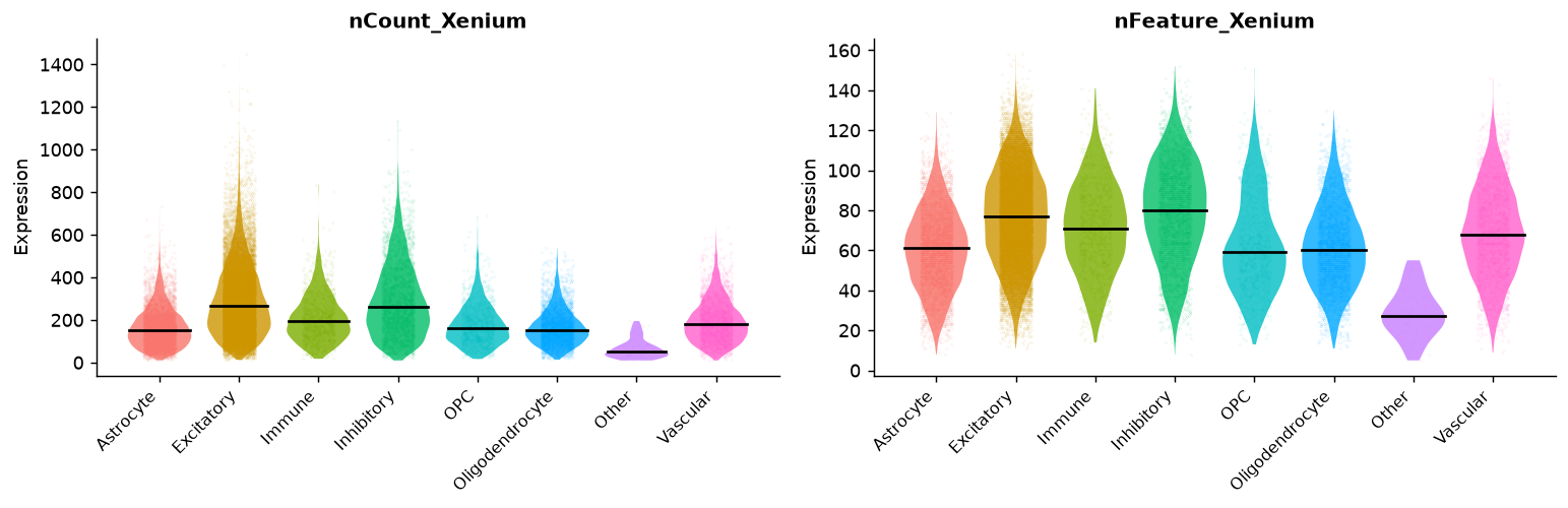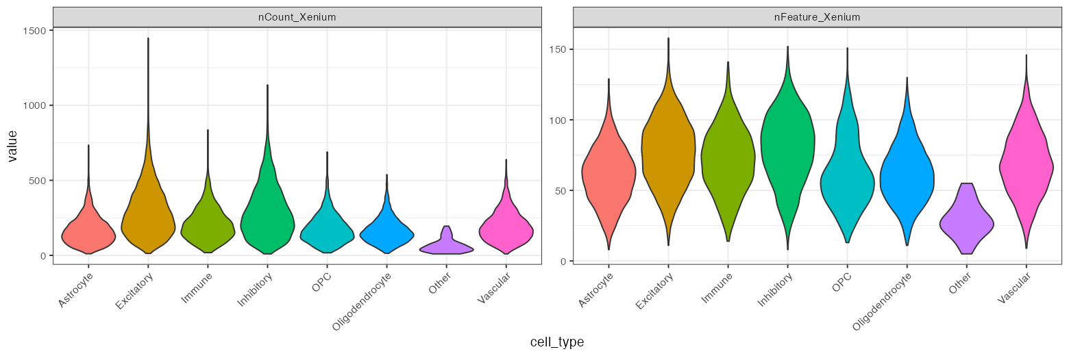
Post-filter QC per cell type (nCount_Xenium / nFeature_Xenium); the cell types come from Step 3. subset() filters the assay, metadata and the spatial centroids together, so every downstream spatial function stays aligned.

Step 3 · Cell types from marker panels¶

A deterministic classifier: each cell is assigned to the cell type whose canonical marker panel it expresses most (arg-max of summed raw counts). Because it is a pure function of the identical count matrix, R and Python produce byte-identical labels — the anchor for every spatial comparison that follows (the same idea as the internal KIT+ TPSAB1+ mast-cell rule).

R (Seurat) Python (Truecell)

markers <- list(
  Excitatory = c("Slc17a7","Slc17a6","Satb2","Fezf2","Neurod6"),
  Inhibitory = c("Gad1","Gad2","Pvalb","Sst","Vip","Lamp5"),
  Astrocyte  = c("Aqp4","Gfap","Ntsr2"),
  Oligodendrocyte = c("Sox10","Opalin","Gjc3"),
  OPC        = c("Pdgfra","Cspg4"),
  Vascular   = c("Cldn5","Pecam1","Kdr","Emcn","Adgrl4"),
  Immune     = c("Cd68","Trem2","Siglech","Laptm5","Cd53"))

cmat  <- GetAssayData(obj, layer = "counts")
score <- sapply(markers, \(g)
           Matrix::colSums(cmat[intersect(g, rownames(cmat)), ]))
best  <- max.col(score, ties.method = "first")
ct    <- names(markers)[best]
ct[apply(score, 1, max) == 0] <- "Other"
obj$cell_type <- ct

CELLTYPE_MARKERS = {
    "Excitatory": ["Slc17a7","Slc17a6","Satb2","Fezf2","Neurod6"],
    "Inhibitory": ["Gad1","Gad2","Pvalb","Sst","Vip","Lamp5"],
    "Astrocyte":  ["Aqp4","Gfap","Ntsr2"],
    "Oligodendrocyte": ["Sox10","Opalin","Gjc3"],
    "OPC":        ["Pdgfra","Cspg4"],
    "Vascular":   ["Cldn5","Pecam1","Kdr","Emcn","Adgrl4"],
    "Immune":     ["Cd68","Trem2","Siglech","Laptm5","Cd53"],
}
counts = obj.assays["Xenium"].layer_data("counts").tocsr()
feats  = {g: i for i, g in enumerate(obj.assays["Xenium"].features())}
score  = np.column_stack([
    counts[[feats[g] for g in gs if g in feats], :].sum(0).A1
    for gs in CELLTYPE_MARKERS.values()])
best   = score.argmax(1)
ct     = np.where(score.max(1) > 0,
                  np.array(list(CELLTYPE_MARKERS))[best], "Other")
obj.meta_data["cell_type"] = ct

Identical counts in both:

cell_type	n	cell_type	n
Excitatory	18,044	Oligodendrocyte	3,570
Astrocyte	5,513	Vascular	3,016
Inhibitory	3,759	Immune	1,311
OPC	1,157	Other	49

Step 4 · Normalise, cluster, UMAP (unsupervised view)¶

R (Seurat) Python (Truecell)

obj <- NormalizeData(obj)
obj <- FindVariableFeatures(obj, nfeatures = 248)
obj <- ScaleData(obj, features = rownames(obj))
obj <- RunPCA(obj, features = rownames(obj), npcs = 30)
obj <- FindNeighbors(obj, dims = 1:20)
obj <- FindClusters(obj, resolution = 0.3)
obj <- RunUMAP(obj, dims = 1:20)

normalize_data(obj, normalization_method="LogNormalize",
               scale_factor=10000)
find_variable_features(obj, selection_method="vst", nfeatures=248)
genes = obj.assays["Xenium"].features()
scale_data(obj, features=genes)
run_pca(obj, n_pcs=30, features=genes, reduction_name="pca")
find_neighbors(obj, dims=range(20), k_param=20)
find_clusters(obj, resolution=0.3, algorithm=1, random_seed=0)
run_umap(obj, dims=range(20), reduction_name="umap", seed=42)

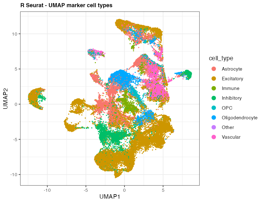
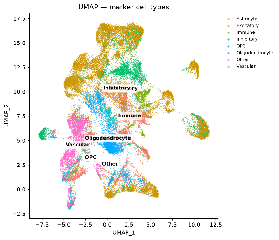
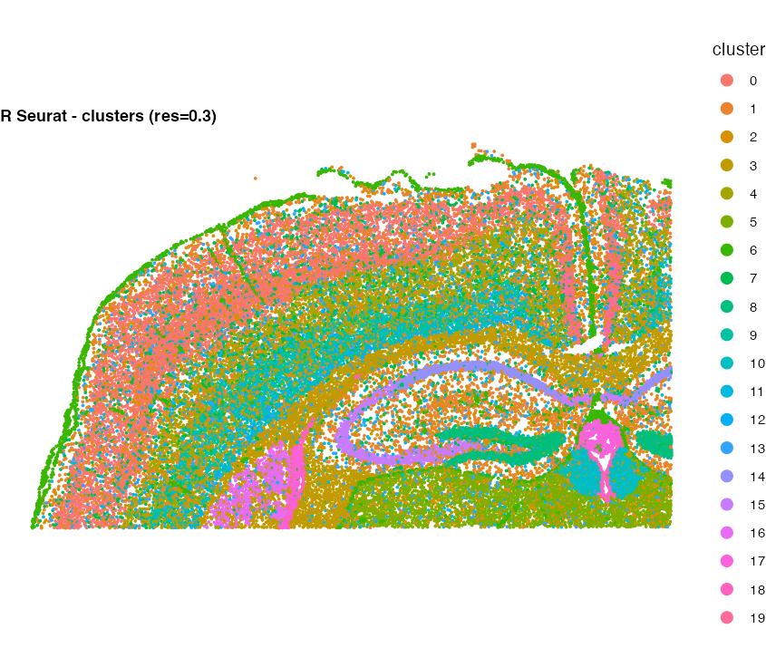
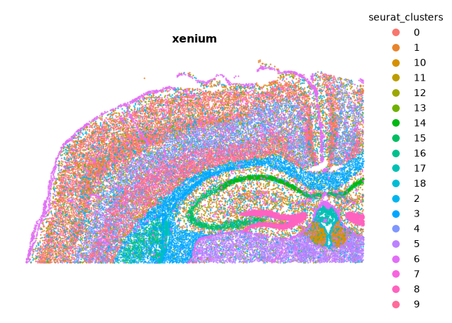
Top row: the UMAP coloured by cell type. Bottom row: the raw unsupervised clusters drawn back in tissue space (ImageDimPlot by cluster) — the cortical layers and hippocampal structure fall out on their own. Louvain clustering is stochastic and the two UMAP libraries (uwot vs umap-learn) place clusters differently — R found 20 clusters, Truecell 18 — but the same spatial structure separates cleanly in both (see the PBMC 3k note).

Step 5 · Cells in tissue space — `ImageDimPlot`¶

R (Seurat)	Python (Truecell)
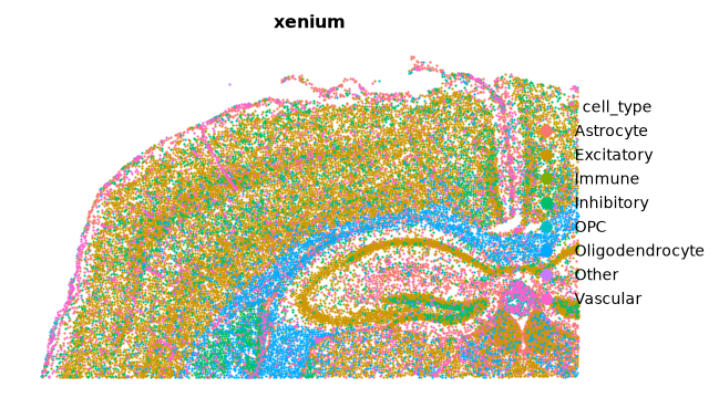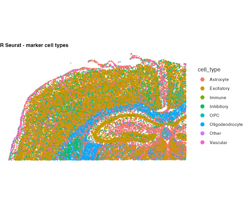
`ImageDimPlot(obj, group.by = "cell_type", size = 1.5)`	`fig = image_dim_plot(obj, group_by="cell_type", size=1.5) fig.savefig("image_celltype.png", dpi=130)`

Both recover the same anatomy: excitatory neurons filling the cortex, oligodendrocytes tracing the white-matter tracts, and the hippocampal formation clearly outlined. Note — under ggplot2 4.x, Seurat's ImageDimPlot renders blank; the R panel here is drawn from GetTissueCoordinates() with geom_point. Truecell's image_dim_plot draws centroids directly with matplotlib, so it is immune to that issue.

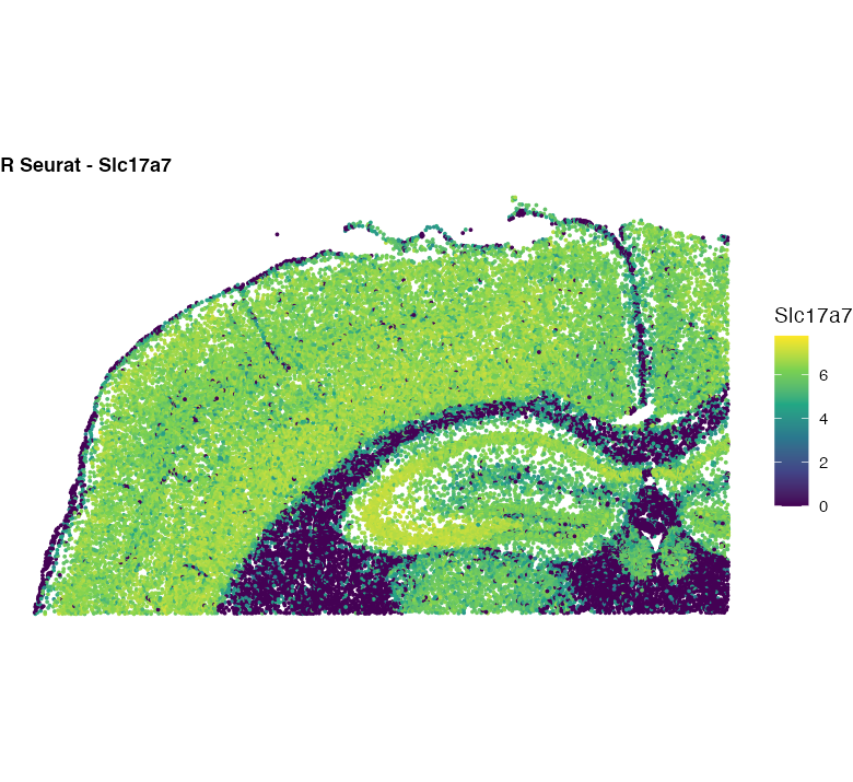
Step 6 · A gene in tissue space — `ImageFeaturePlot`¶

R (Seurat)	Python (Truecell)
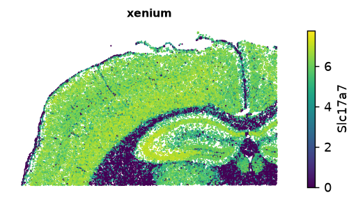`ImageFeaturePlot(obj, features = "Slc17a7")`	`fig = image_feature_plot(obj, "Slc17a7", cmap="viridis")`

Slc17a7 (VGLUT1) marks excitatory neurons — bright across cortex, dark in the white matter and ventricles, in both implementations.

Step 7 · Tissue coordinates & nearest-neighbour distance¶

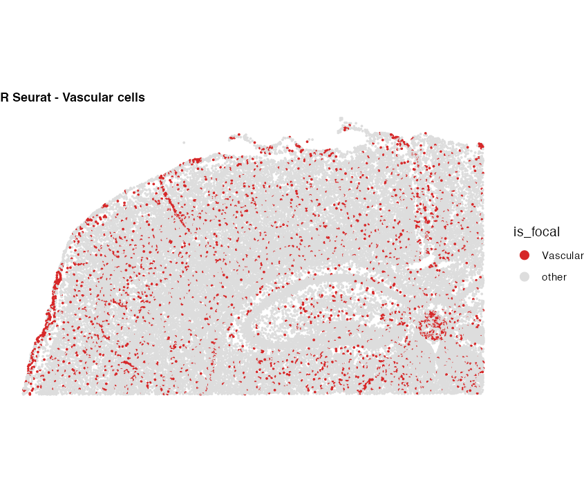
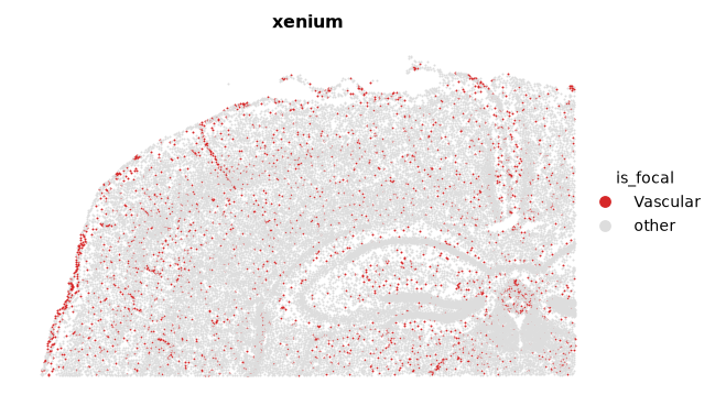
We treat Vascular cells as the focal population (the analog of mast cells in the internal analysis) and measure, per cell, the distance to its nearest other vascular cell. Seurat users reach for FNN::get.knn; Truecell wraps the identical KD-tree in nearest_neighbor_distance.

R (Seurat) Python (Truecell)

xy  <- GetTissueCoordinates(obj)[, c("x","y")]
foc <- xy[obj$cell_type == "Vascular", ]

# distance to nearest *other* vascular cell
d <- FNN::get.knn(foc, k = 1)$nn.dist[, 1]
median(d)   # 24.0739 µm

coords = get_tissue_coordinates(obj)   # x, y, cell, image

nn = nearest_neighbor_distance(obj, "cell_type", "Vascular")
nn["distance"].median()                # 24.0739 µm

metric	R Seurat (FNN)	Truecell
n Vascular	3,016	3,016
nearest-neighbour median	24.0739 µm	24.0739 µm
nearest-neighbour mean	30.5612 µm	30.5612 µm

Step 8 · Local neighbourhood density¶

For every vascular cell, what fraction of its 10 nearest neighbours are also vascular? (Local "clumpiness" of the focal type.)

R (Seurat) Python (Truecell)

knn  <- FNN::get.knnx(xy, foc, k = 11)$nn.index[, -1]  # drop self
prop <- rowMeans(matrix((obj$cell_type == "Vascular")[knn],
                        nrow = nrow(foc)))
mean(prop)     # 0.18107

nb = local_neighborhood(obj, "cell_type",
                        reference="Vascular", k=10)
nb["prop_Vascular"].mean()      # 0.18107

Both give a mean local vascular density of 0.18107 — 8-figure agreement.

Step 9 · Composition test across a spatial region¶

Split the section into dorsal / ventral halves (median y) and test which cell types are enriched where. Seurat users build this table by hand (Fisher + p.adjust); Truecell packages it as composition_test.

R (Seurat) Python (Truecell)

obj$region <- ifelse(obj$y >= median(obj$y),
                     "ventral", "dorsal")
tab <- table(obj$cell_type, obj$region)
# per cell type: Fisher (group vs rest), log2 ratio, BH
# ... (a dozen lines of bookkeeping) ...

obj.meta_data["region"] = np.where(
    coords["y"].values >= coords["y"].median(),
    "ventral", "dorsal")

comp = composition_test(obj, group_by="cell_type",
                        split_by="region", reference="dorsal")
comp.attrs["chisq_p"]     # 1.14e-163

Identical enrichment in both (log2 > 0 ⇒ enriched ventral):

cell_type	log2 ratio	BH padj	enriched in
Other	+1.180	1.2e-02	ventral
OPC	+1.037	8.5e-33	ventral
Astrocyte	+0.748	8.5e-93	ventral
Oligodendrocyte	+0.279	2.3e-09	ventral
Vascular	+0.059	0.281 (ns)	ventral
Immune	+0.051	0.536 (ns)	ventral
Excitatory	−0.267	9.3e-68	dorsal
Inhibitory	−0.448	3.4e-23	dorsal

Overall χ² p = 1.14e-163 in both. Neurons concentrate dorsally (cortex); glial/progenitor types (OPC, astrocyte, oligodendrocyte) skew ventrally. composition_test reports a sample odds ratio (a·d / b·c); R's fisher.test returns the conditional-MLE odds ratio — they differ in the 4^th decimal by definition, but the log2 ratios and p-values are identical.

Step 10 · Niche analysis — `BuildNicheAssay`¶

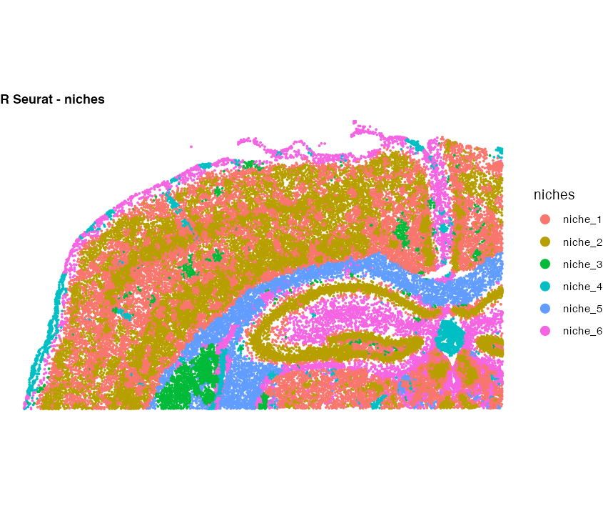
Cluster cells by the composition of their spatial neighbourhood into spatial "niches" (Seurat v5's BuildNicheAssay).

R (Seurat) Python (Truecell)

obj <- BuildNicheAssay(obj, fov = "fov",
                       group.by = "cell_type",
                       niches.k = 6, neighbors.k = 20)
ImageDimPlot(obj, group.by = "niches")

build_niche_assay(obj, "cell_type",
                  k=20, niches=6, seed=0)
fig = image_dim_plot(obj, group_by="niches", size=1.5)

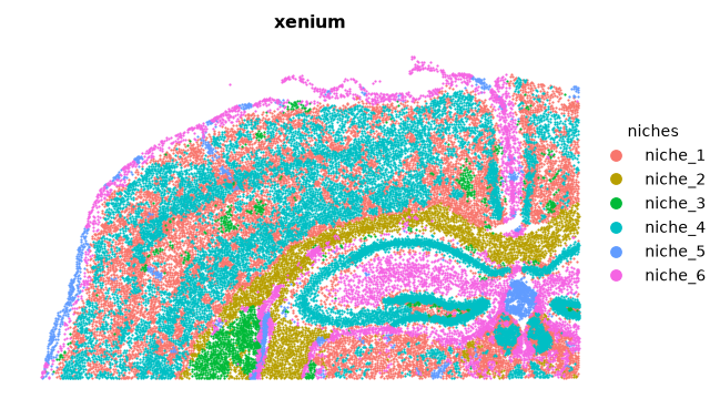Both build a neighbourhood-composition matrix and k-means it into niches. The k-means initialisation differs between R and Python so niche labels differ, but both partition the section into the same spatial domains — cortical layers, white matter, and hippocampal subfields.

Parity — verified against R Seurat¶

Cross-checked by compare_xenium_anchors.py (R reference ↔ Truecell). Every deterministic anchor matches to 8 significant figures:

anchor	R Seurat	Truecell
cells (raw / QC)	36,602 / 36,419	36,602 / 36,419	✓
genes	248	248	✓
cell-type counts (×8)	exact	exact	✓
Vascular nearest-neighbour median	24.073884	24.073884	✓
Vascular nearest-neighbour mean	30.561227	30.561227	✓
Vascular local density mean	0.18106764	0.18106764	✓
composition log2 ratios (×8)	exact	exact	✓
composition Fisher p / BH padj	exact	exact	✓
composition χ² p	1.138165e-163	1.138165e-163	✓
clusters / niches (stochastic)	20 / 6	18 / 6	structure

Quick Reference — Spatial API Translation¶

Task	R (Seurat)	Python (Truecell)
Load Xenium	`LoadXenium(dir)`	`load_xenium(dir)`
Load Visium / CosMx	`Load10X_Spatial` / `LoadNanostring`	`load_visium` / `load_cosmx`
Tissue coordinates	`GetTissueCoordinates(obj)`	`get_tissue_coordinates(obj)`
Spatial k-NN	`FNN::get.knn` / `get.knnx`	`spatial_knn(coords, k, query)`
Nearest-type distance	`FNN::get.knn` idiom	`nearest_neighbor_distance(obj, group_by, ref)`
Neighbourhood composition	(hand-rolled)	`local_neighborhood(obj, group_by, ref, k)`
Niche clustering	`BuildNicheAssay(obj, fov, group.by)`	`build_niche_assay(obj, group_by, k, niches)`
Composition / enrichment	(hand-rolled Fisher + `p.adjust`)	`composition_test(obj, group_by, split_by)`
Cells in space	`ImageDimPlot(obj, group.by)`	`image_dim_plot(obj, group_by)`
Feature in space	`ImageFeaturePlot(obj, features)`	`image_feature_plot(obj, feature)`

Reproducing this tutorial¶

git clone https://github.com/GenomicAI/truecell.git
cd truecell
git checkout feature/spatial-seurat-parity
uv venv && source .venv/bin/activate
uv pip install -e ".[analysis]"

# 1. Python side (auto-downloads the ~20 MB dataset) — writes figures_spatial/
python tutorials/generate_spatial_plots.py

# 2. R reference figures + figures_spatial/r_reference.json
#    (needs Seurat, FNN, ggplot2, jsonlite; reads the cache from step 1)
Rscript tutorials/xenium_spatial_verify.R

# 3. Print the R-vs-Python parity table shown above
python tutorials/compare_xenium_anchors.py

All three scripts live in tutorials/ and read/write tutorials/figures_spatial/, so the whole comparison is self-contained.

References¶

10x Genomics (2023). Xenium In Situ — Fresh Frozen Mouse Brain (Coronal), CTX + HP subset. https://www.10xgenomics.com/datasets

Hao Y, et al. (2024). Dictionary learning for integrative, multimodal and scalable single-cell analysis. Nature Biotechnology 42, 293–304.

Seurat spatial vignette (Xenium): https://satijalab.org/seurat/articles/spatial_vignette_2

Xenium Spatial Tutorial — R Seurat vs Truecell (Python)¶

Setup¶

Step 1 · Load the Xenium output¶

Step 2 · QC filter¶

Step 3 · Cell types from marker panels¶

Step 4 · Normalise, cluster, UMAP (unsupervised view)¶

Step 5 · Cells in tissue space — ImageDimPlot¶

Step 6 · A gene in tissue space — ImageFeaturePlot¶

Step 7 · Tissue coordinates & nearest-neighbour distance¶

Step 8 · Local neighbourhood density¶

Step 9 · Composition test across a spatial region¶

Step 10 · Niche analysis — BuildNicheAssay¶

Parity — verified against R Seurat¶

Quick Reference — Spatial API Translation¶

Reproducing this tutorial¶

References¶

Step 5 · Cells in tissue space — `ImageDimPlot`¶

Step 6 · A gene in tissue space — `ImageFeaturePlot`¶

Step 10 · Niche analysis — `BuildNicheAssay`¶