Spatial Statistics and the Spatial Container — R Seurat vs Truecell (Python)
Wave 2's last side-by-side, and the first one to check two things the existing
Xenium tutorial left alone: the container —
FOV, Centroids, Segmentation — and the one real spatial statistic in
the library, FindSpatiallyVariableFeatures. Every R Seurat call is paired with
the Truecell equivalent and both outputs are shown side by side.
Dataset: 10x Xenium mouse brain, coronal CTX + HP section. 36,602 cells × 248 genes, one FOV. Auto-downloads (~14 MB). R reference: Seurat 5.5.1 / SeuratObject 5.4.0 · Python: Truecell
| Seurat | Truecell |
|---|---|
LoadXenium(dir, molecule.coordinates = FALSE) |
load_xenium(dir) |
CreateCentroids(coords) |
create_centroids(coords) |
CreateFOV(coords, type = "centroids") |
create_fov(coords, type_="centroids") |
CreateSegmentation(coords) |
create_segmentation(coords) |
GetTissueCoordinates(fov) · Radius(centroids) |
fov.get_tissue_coordinates() · centroids.radius() |
FindSpatiallyVariableFeatures(obj, selection.method = "moransi") |
find_spatially_variable_features(obj, method="moransi") |
This tutorial found and fixed three defects. Moran's I was computed on a k-nearest-neighbour graph rather than Seurat's row-standardised inverse-square weights, so it answered a different question under the same name.
Centroidsnever received a radius, which silently disabled every true-to-scale spot renderer. AndSegmentationstored polygons open where R closes them. Two further divergences are left standing on purpose, and the reasoning is written up in what this tutorial found.
Headline
| Metric | Result |
|---|---|
| Anchors matching Seurat exactly | 39 / 39 |
| Moran's I per gene vs R (248 genes, 2,000 cells) | max abs diff 1.6e-14, Pearson 1.0000000000 |
| Moran's I — Seurat's top 10 recovered | 10 / 10, in the same order |
| Before the fix — kNN weighting vs R | Pearson 0.986, but 7/10 top genes and a median 1.23× bias |
Centroids.radius() — auto radius vs .AutoRadius |
42.82543 vs 42.82543 |
Segmentation ring vertices (square, per cell) |
5 vs 5 |
| Full-slide Moran's I, R's exact weights | 5.3 s, 0.95 GB — Seurat needs a 10.7 GB dense matrix |
The last anchor to match was GetTissueCoordinates' shape: truecell carried the
cell only as the row label until its frame gained the cell column R returns.
Setup
| R (Seurat) | Python (Truecell) |
|---|---|
molecule.coordinates = FALSE is not optional on the public cache: it ships the
cell-feature matrix and cells.csv.gz but no transcripts.parquet, and
LoadXenium raises rather than skipping the molecules. load_xenium reads the
same directory and simply leaves molecules empty — the first of several places
where the two loaders are permissive about different things.
Both read 36,602 cells × 248 genes, with identical cell and feature names in identical order (the name digests match).
What is in the object
| R (Seurat) | Python (Truecell) |
|---|---|
The FOV is filed under the same name as well: load_xenium takes LoadXenium's
fov argument with the same default, so R code indexing obj[["fov"]] carries
over as obj.images["fov"]. Until the loaders were checked against Seurat's
readers it was always "xenium", with no way to choose.
Radius() on the FOV is empty in both tools — that is R's design, and the
number lives on the boundary underneath. Getting that right matters more than it
looks: truecell's plotting code read the radius off the FOV, so it always saw
None. See defect 2.
R routes the control probes into three extra assays (BlankCodeword,
ControlCodeword, ControlProbe — 225 / 41 / 27 features). load_xenium drops
them by default and keep_controls=True keeps all 541 rows in the one assay
instead. A documented difference in shape, not in content.
The constructors
Small enough to check by eye, which is the point — the slide-scale anchors say whether the tools agree, these say what they agree on.
| R (Seurat) | Python (Truecell) |
|---|---|
0.165 is SeuratObject's .AutoRadius: 0.01 × mean(width, height) of the
bounding box, so 0.01 × mean(3, 30). truecell returned None here before this
tutorial.
Polygons are where the two most visibly parted company:
| R (Seurat) | Python (Truecell) |
|---|---|
Spatially variable features
This is the section the tutorial exists for.
| R (Seurat) | Python (Truecell) |
|---|---|
The statistic agrees to 1.6e-14 across all 248 genes and the top ten come out in the same order. The p-values do not agree, and that is deliberate — see the two differences left standing.
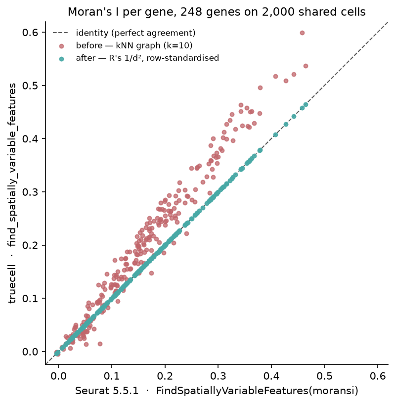
A note on scale. RunMoransI builds as.matrix(dist(pos)) — the full n × n
weight matrix. On this slide that is a 10.7 GB allocation, which is why the
comparison above runs on a shared 2,000-cell subset. truecell evaluates the same
weights in row blocks and runs the whole slide in 5.3 s at 0.95 GB peak. The
answers are R's; the ceiling is not.
What this tutorial found
1. Moran's I was built on the wrong weight matrix
Seurat's RunMoransI constructs weights <- 1 / pos.dist.mat ^ 2 over every
pair of cells, and Rfast2::moranI row-standardises it before computing
cor(y, x) · sd(y) / sd(x). truecell used a k-nearest-neighbour graph with
k = 10.
Both are legitimate Moran's I. Only one is the one the function said it was computing, and a Moran's I is defined relative to its weights — change them and you change the answer.
What made it survive is that it is a good approximation. Pearson 0.986 against R, Spearman 0.982, 46 of R's top 50 genes. Nothing about it looks wrong in a plot. But it runs a median 1.23× high, differs by up to 0.14 in absolute I, and recovers only 7 of R's top 10 — and the top of the ranking is the entire output anyone reads off this function.
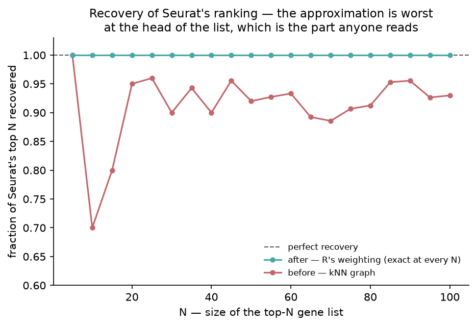
Fixed by making R's weighting the default, evaluated in row blocks so the n × n
matrix is never materialised. weights="knn" still selects the old behaviour for
slides where the O(n²) pass is genuinely too slow, now documented as the
approximation it is. After the fix: max abs diff 1.6e-14, 10/10.
2. Centroids never carried a radius
SeuratObject always computes one — .AutoRadius, 1% of the mean bounding-box
dimension, 42.83 on this slide. truecell left the slot None.
The consequence was invisible. _spot_collection returns None for a None
radius and the caller falls back to a fixed-size scatter, so every true-to-scale
spot renderer silently stopped being true-to-scale on every FOV that did not
come from a Visium scalefactors_json.json. No warning, no exception; the plots
simply stopped meaning what they claimed. This is the same shape as T-obj's
FetchData bug — a function returning something plausible rather than something
right.
Two things were wrong, and only fixing both helps: Centroids did not compute
the radius, and _spatial_panel read it off the FOV, where it is None in R
too. It now reads the default boundary, which is where R keeps it.
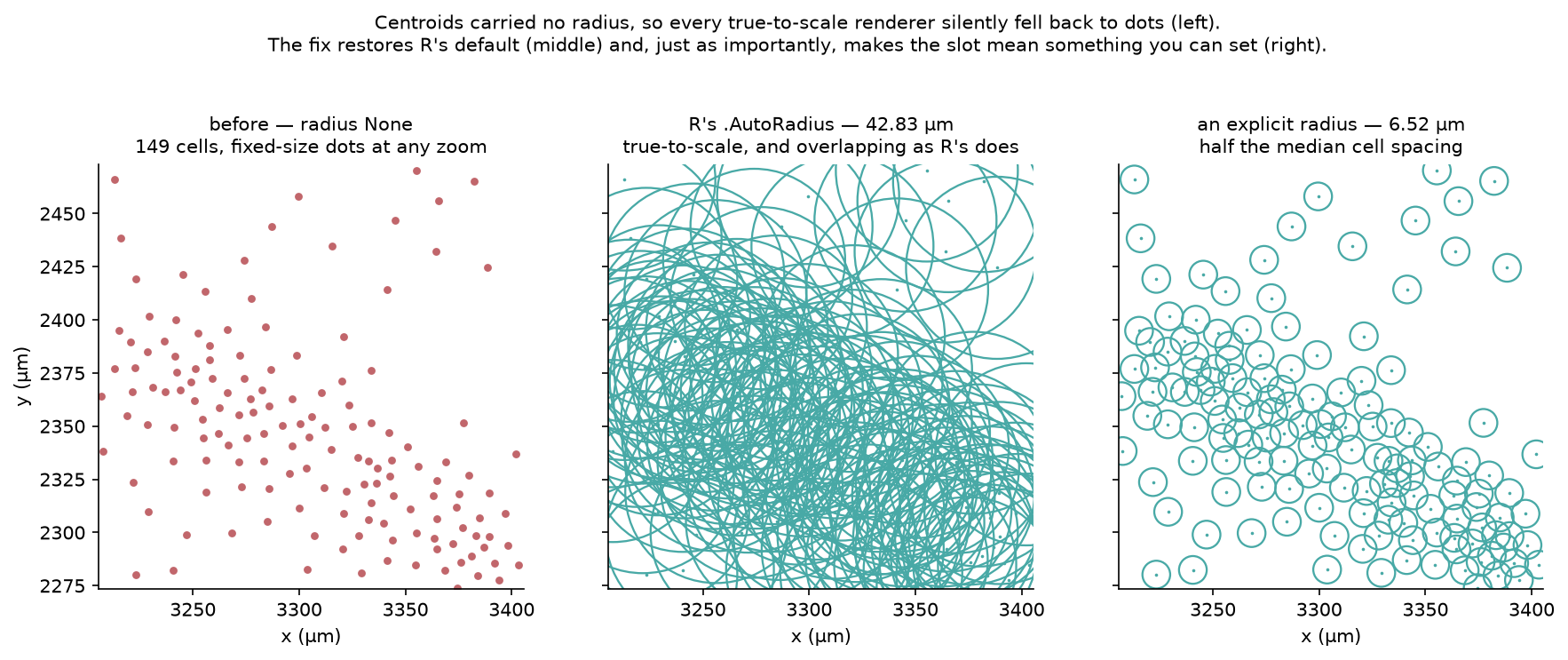
The middle panel is worth dwelling on. R's default radius overlaps badly at this cell density, because 1% of a bounding box is a slide-scale hint and not a measurement of a cell. Seurat draws this slide the same way. The fix is not that truecell now draws prettier spots — it is that the slot means something, and can be set.
3. Segmentation stored polygons open
R closes each ring by repeating the first vertex: a four-vertex square comes back as five rows. truecell stored four.
Anything that measures a perimeter from the vertex list, or strokes an outline without asking the renderer to close the path, is short exactly one edge. Fixed, and idempotent — an already-closed ring is left alone. Concave shapes survive: an L-shape goes in with six vertices and comes back with seven, notch intact, in both tools.
R also traverses the ring in the opposite direction. That is the same polygon described backwards, so it is left alone.
Two differences left standing
The Moran's I p-value. R runs a 999-permutation test through
Rfast2::moranI. On this 248-gene panel that produces 14 distinct p-values
and ties 233 of 248 genes at its floor of 1/1025 — it cannot tell the most
spatially variable gene in the panel from the two-hundredth. truecell's
normal-approximation p-value is continuous, deterministic and the standard
closed form for Moran's I. Matching R would have cost real information and bought
nothing, so the statistic was fixed and the p-value deliberately was not.
This is the one judgement call in the tutorial, and it cuts the other way from
T-sk's project_data, where the better-scoring implementation was the wrong one
because it cost what the API existed to provide. The test is not "which number is
nicer" — it is whether the divergence costs the user something they came for.
Here it does not.
The FOV Key. R derives it from the assay (CreateFOV(coords, assay="RNA")
gives RNA_); truecell hardcodes fov_. It appears in __repr__ and nowhere
else — no lookup, no prefixing, no FetchData path — so changing a default to
correct a display string was not worth the churn. Recorded rather than fixed.
The anchor that used to differ
GetTissueCoordinates returns three columns in R (x, y, cell). truecell
returned two and carried the cell only as the DataFrame index, and that was the
one anchor that did not match. get_tissue_coordinates() on a Centroids,
Segmentation or FOV now returns the cell column too, the frame R returns, so
all 39 anchors match.
Parity — verified against R Seurat
| Section | Anchors | Matching | Tolerance |
|---|---|---|---|
container — cells, features, boundaries, radius, coordinate frame |
22 | 22 | exact except 3 float anchors |
toy — the constructors on 4 cells and 2 squares |
10 | 10 | exact except auto_radius |
moransi — top genes, I values, ranking digest |
7 | 7 | exact except 3 float anchors |
| Total | 39 | 39 |
Thirty-two of the thirty-nine anchors are compared with no tolerance at all —
names, orders, counts, digests, boundary sets, vertex counts. The seven floating
point ones are named individually in FLOAT_TOLERANCES rather than covered by a
blanket rule, so a new anchor cannot inherit slack nobody chose for it.
Running it
# 1. Python side — writes figures_svf/py_anchors.json and cells.txt
python tutorials/xenium_svf_tutorial.py

# 2. R side — writes figures_svf/r_anchors.json (needs Rfast2)
Rscript tutorials/xenium_svf_verify.R

# 3. Compare
python tutorials/xenium_svf_tutorial.py --report

# 4. Figures
python tutorials/generate_svf_plots.py
The R side needs Rfast2; without it Seurat falls back to ape::Moran.I, a
different estimator, and the comparison would silently be against something other
than Seurat's documented default. The verify script checks for it and stops
rather than producing numbers that look fine and mean something else.