Advanced Tutorial — PBMC 8k Clustering & Subclustering (R Seurat vs Truecell)¶

A more complex companion to the PBMC 3k tutorial. It reproduces the standard Seurat guided-clustering workflow on a larger 10x Genomics dataset (~8,400 PBMCs, GRCh38) and then adds the advanced subclustering step the Seurat reference papers use to resolve fine-grained immune states: the T/NK lymphoid compartment is isolated and re-analysed from scratch to separate naive CD4, memory CD4, CD8, and NK populations that the global clustering merges.

Dataset: 8k PBMCs from a Healthy Donor — 10x Genomics (GRCh38, v2) Python: Truecell v0.2.0 Methodology: Satija et al. 2015 · Butler et al. 2018 · Hao et al. 2021

Scope note. This tutorial stays within the single-assay RNA graph-based clustering workflow these papers established — which is exactly where subclustering shines. SCTransform and multimodal WNN are covered in the other tutorials; anchor-based (CCA/RPCA) integration is not yet ported.

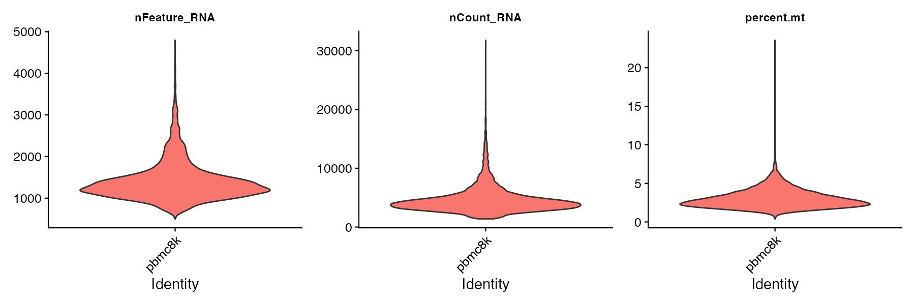
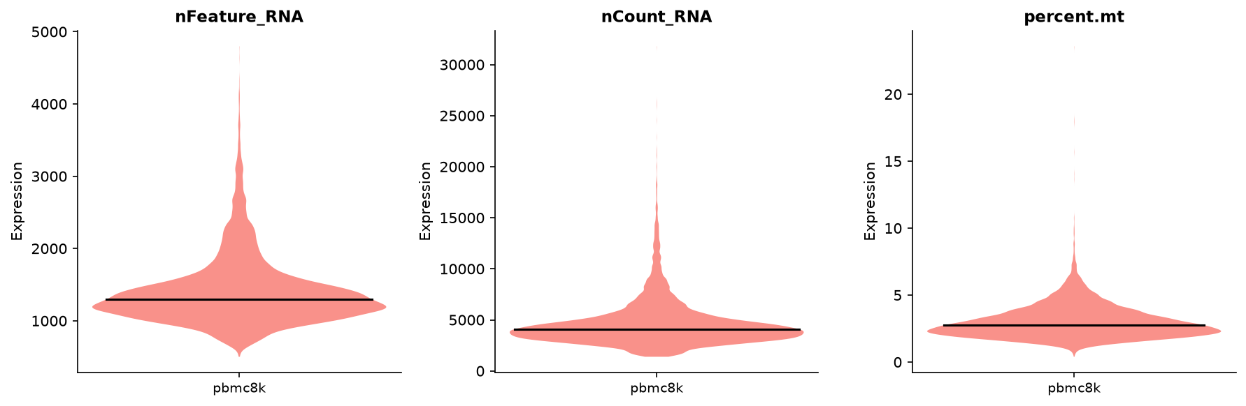
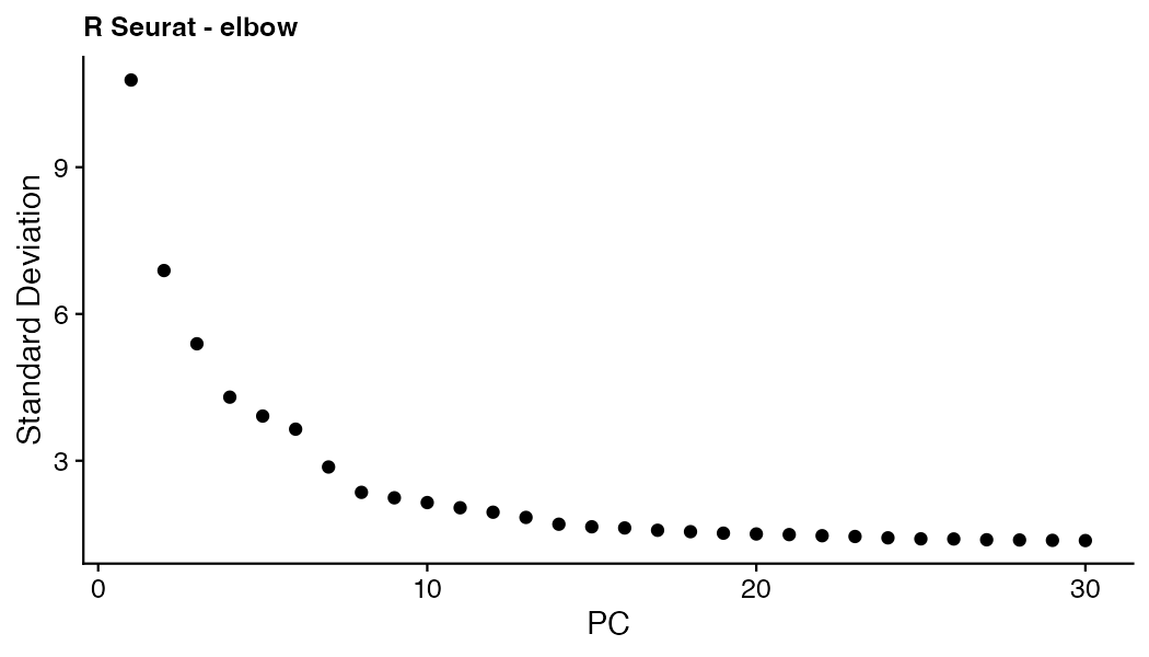
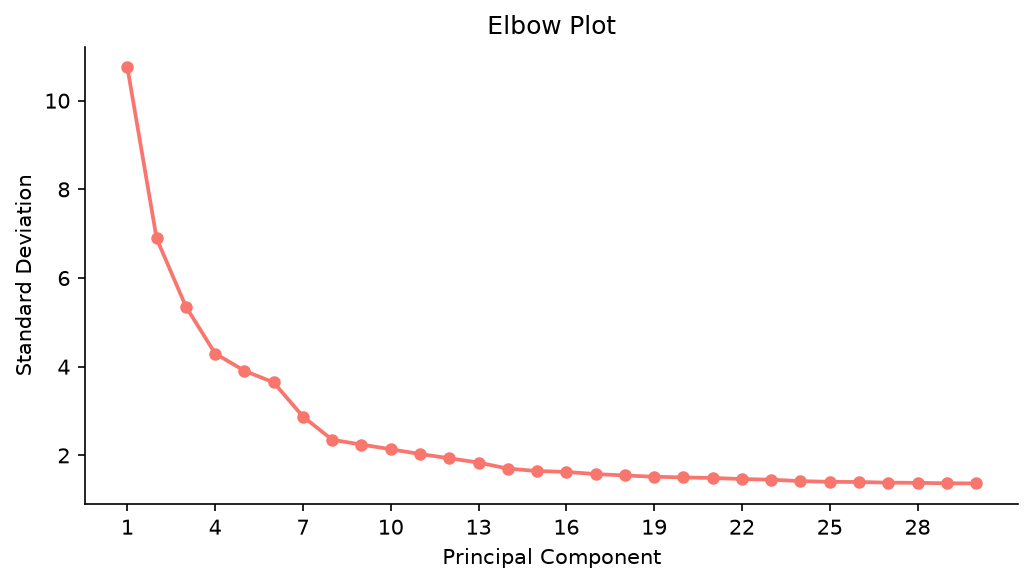
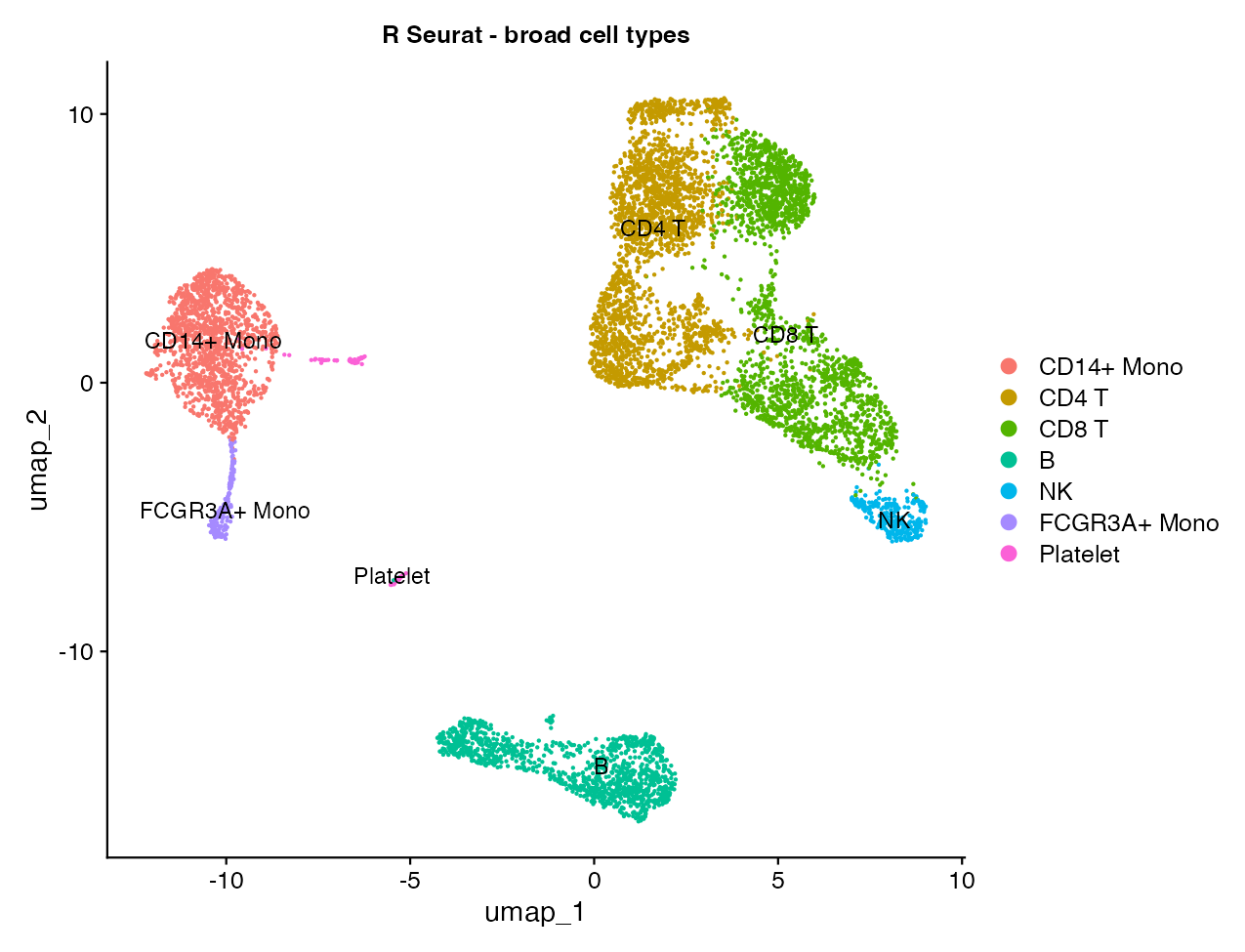
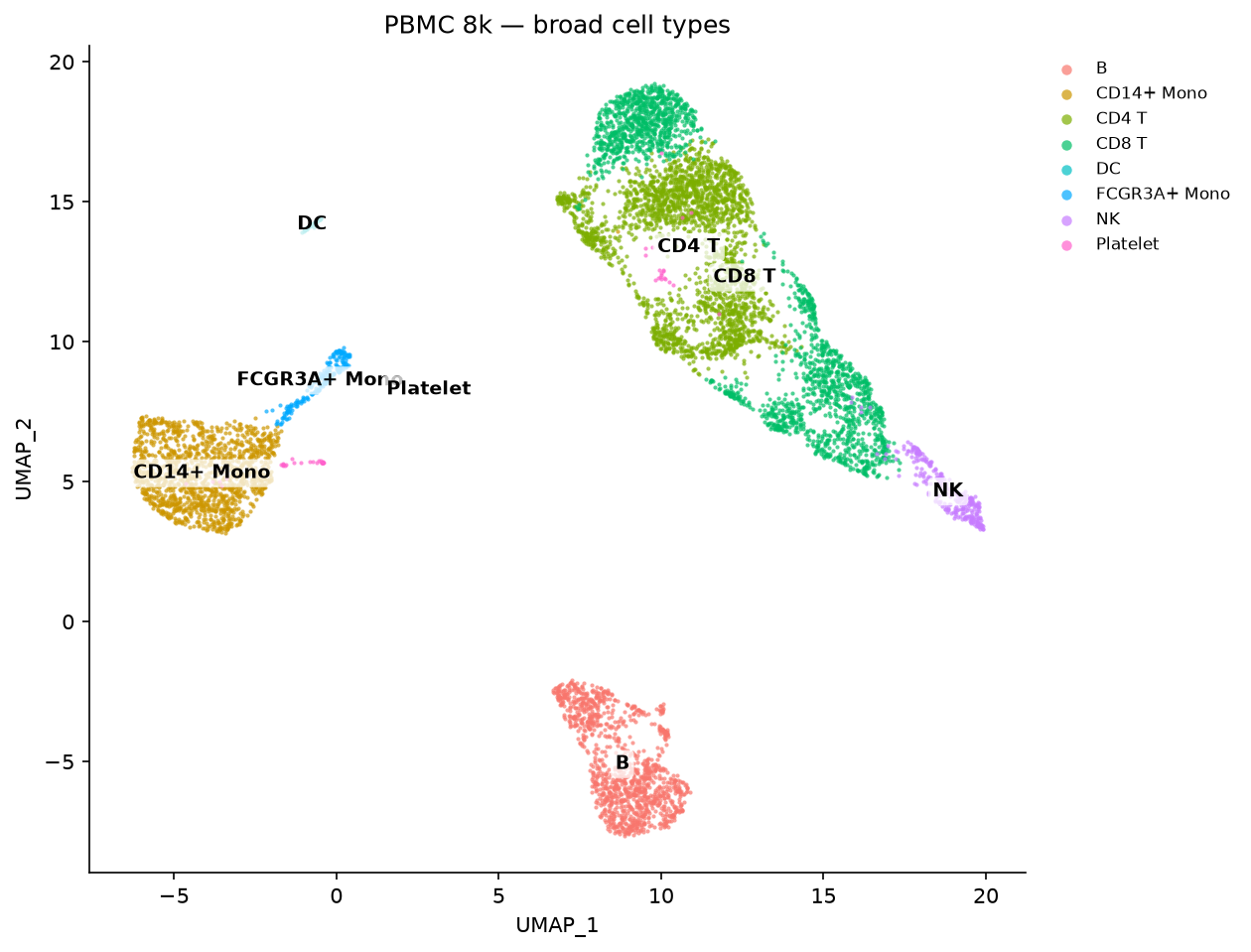
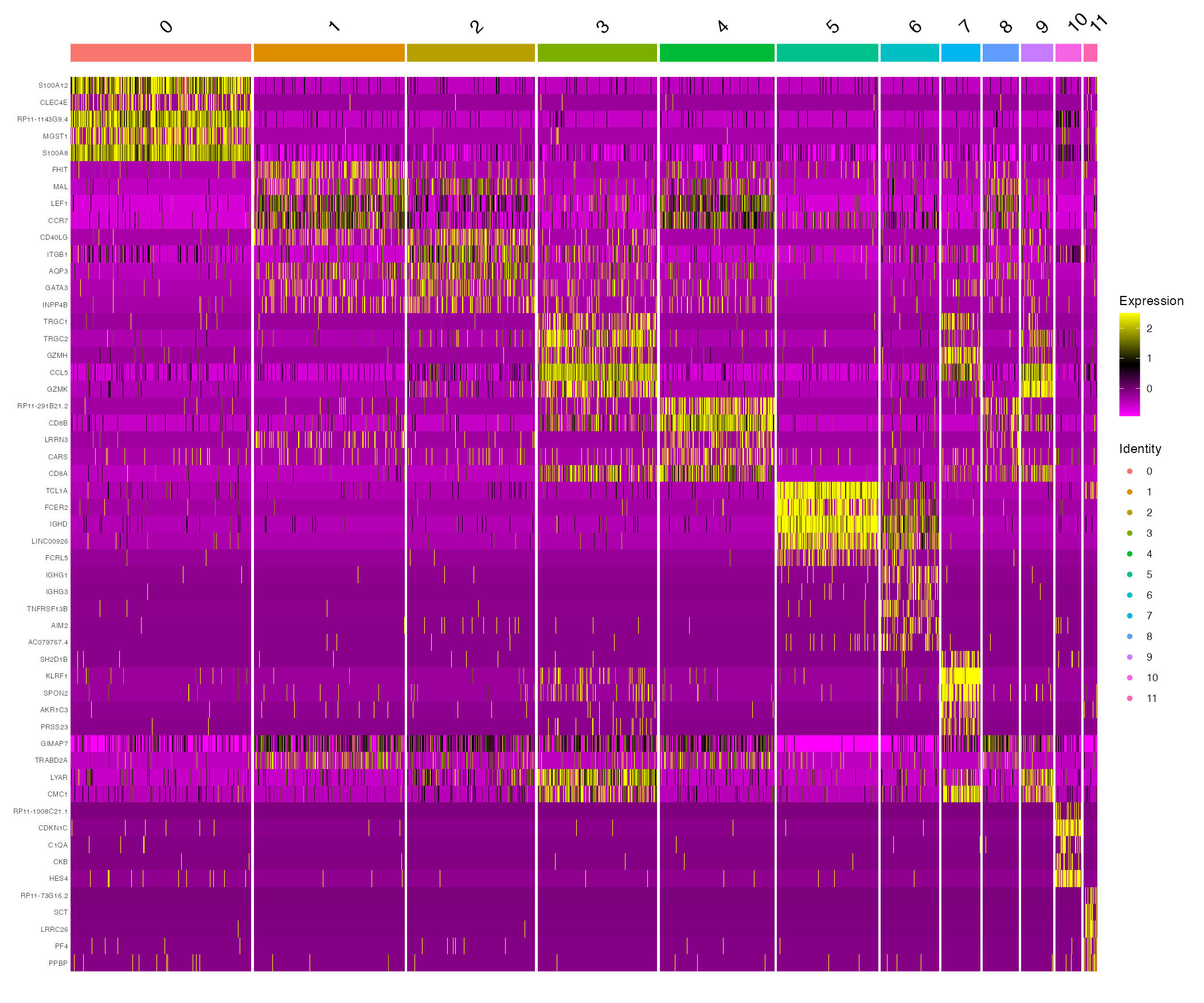
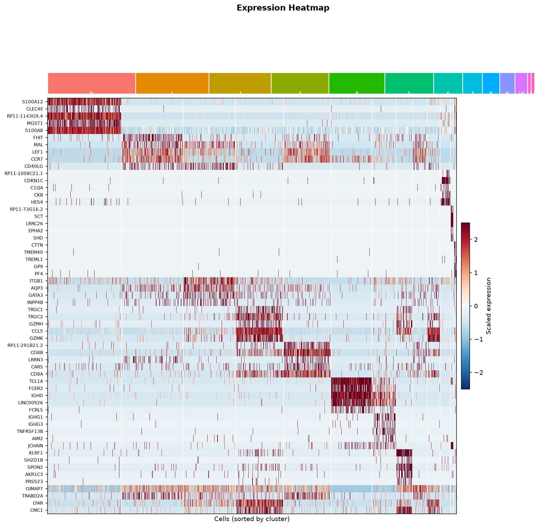
About the figures. Each step shows a genuine side-by-side comparison: the left image is real R Seurat output (pbmc8k_subclustering_verify.R, titled "R Seurat – …") and the right image is Truecell (generate_advanced_plots.py). Both run the identical pipeline and the same two annotation heuristics on the same data; clustering is stochastic and the two UMAP libraries (uwot vs umap-learn) place clusters differently, so compare the structure, not exact positions or cluster numbers.

Run everything with:

python tutorials/pbmc8k_subclustering_tutorial.py   # printed validation
python tutorials/generate_advanced_plots.py         # writes figures_advanced/  (Truecell figures)
Rscript tutorials/pbmc8k_subclustering_verify.R     # writes figures_advanced/r_*  (R Seurat figures)

Step 1 · Load Data & Create Object¶

R (Seurat) Python (Truecell)

library(Seurat)
pbmc.data <- Read10X("pbmc8k/filtered_gene_bc_matrices/GRCh38/")
pbmc <- CreateSeuratObject(
  counts = pbmc.data, project = "pbmc8k",
  min.cells = 3, min.features = 200
)

from truecell.datasets import pbmc8k
from truecell.truecell import create_truecell_object

counts, genes, cells = pbmc8k()          # auto-downloads ~38 MB
pbmc = create_truecell_object(
    counts=counts, project="pbmc8k",
    min_cells=3, min_features=200,
    feature_names=genes, cell_names=cells,
)

Step 2 · QC & Filtering¶

R (Seurat) Python (Truecell)

pbmc[["percent.mt"]] <- PercentageFeatureSet(pbmc, pattern = "^MT-")
VlnPlot(pbmc, c("nFeature_RNA","nCount_RNA","percent.mt"), ncol = 3)

pbmc <- subset(pbmc, subset =
  nFeature_RNA > 200 & nFeature_RNA < 2500 & percent.mt < 5)

from truecell.preprocessing import percentage_feature_set
from truecell.plotting import vln_plot

percentage_feature_set(pbmc, pattern=r"^MT-", col_name="percent.mt")
vln_plot(pbmc, ["nFeature_RNA","nCount_RNA","percent.mt"], ncol=3)

md = pbmc.meta_data
keep = (md["nFeature_RNA"] > 200) & (md["nFeature_RNA"] < 2500) & (md["percent.mt"] < 5)
pbmc = pbmc.subset(cells=list(md.index[keep]))
# 8,381 → 7,475 cells

Step 3 · Normalize → HVG → Scale → PCA¶

R (Seurat) Python (Truecell)

pbmc <- NormalizeData(pbmc)
pbmc <- FindVariableFeatures(pbmc, nfeatures = 2000)
pbmc <- ScaleData(pbmc, features = rownames(pbmc))
pbmc <- RunPCA(pbmc, npcs = 50)
ElbowPlot(pbmc, ndims = 30)

from truecell.preprocessing import normalize_data, find_variable_features, scale_data
from truecell.reduction import run_pca
from truecell.plotting import elbow_plot

normalize_data(pbmc)
find_variable_features(pbmc, selection_method="vst", nfeatures=2000)
scale_data(pbmc, features=pbmc.assays["RNA"]._all_feature_names)
run_pca(pbmc, n_pcs=50, features=pbmc.assays["RNA"].variable_features)
elbow_plot(pbmc, ndims=30)

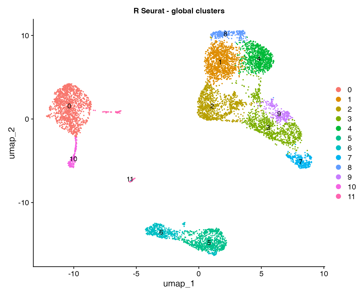
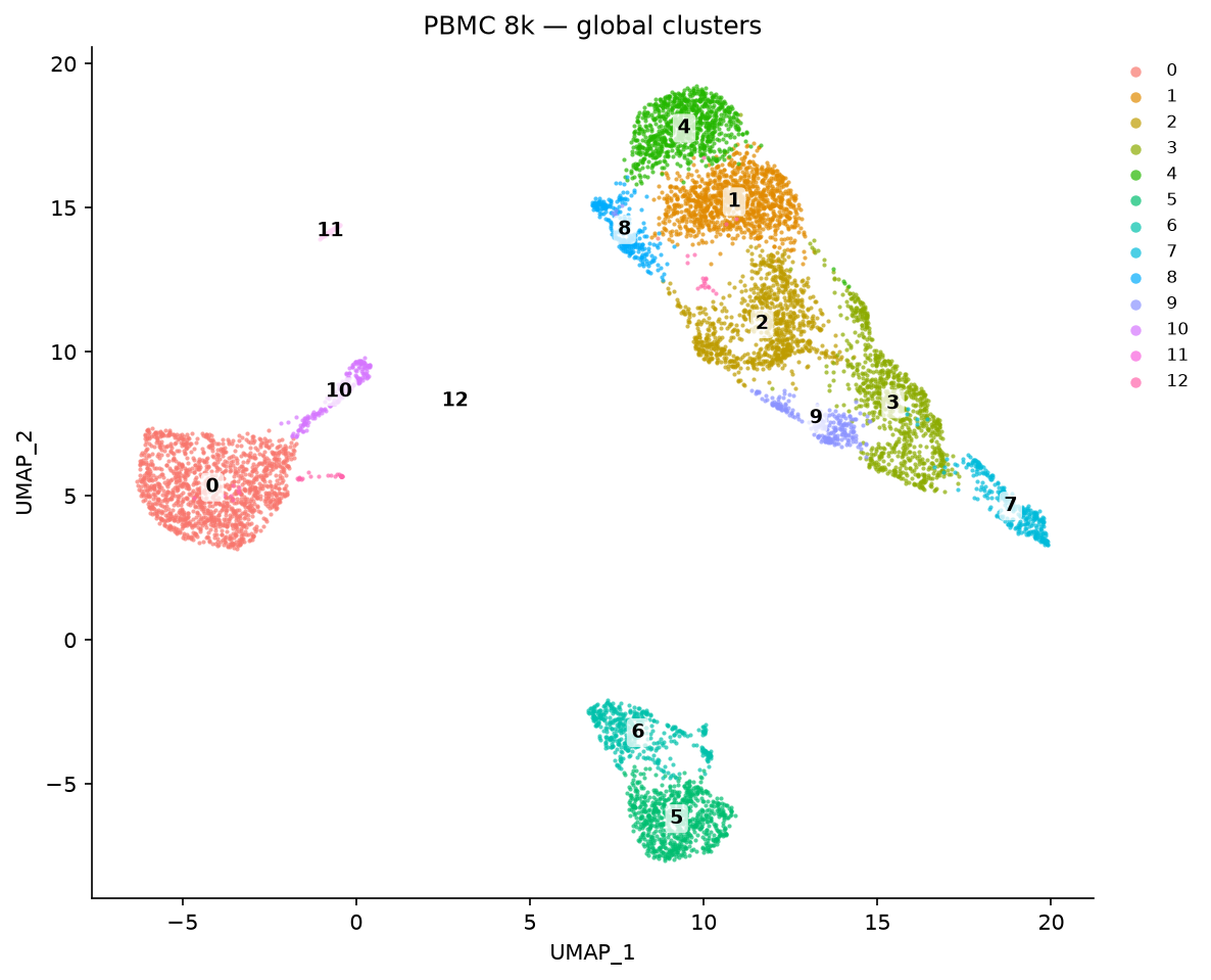
Step 4 · Global Clustering & UMAP¶

R (Seurat) Python (Truecell)

pbmc <- FindNeighbors(pbmc, dims = 1:10)
pbmc <- FindClusters(pbmc, resolution = 0.5)   # 12 clusters
pbmc <- RunUMAP(pbmc, dims = 1:10)
DimPlot(pbmc, reduction = "umap", label = TRUE)

from truecell.neighbors import find_neighbors
from truecell.clustering import find_clusters
from truecell.umap import run_umap
from truecell.plotting import dim_plot

find_neighbors(pbmc, dims=range(10), k_param=20)
find_clusters(pbmc, resolution=0.5, random_seed=0)   # 12 clusters
run_umap(pbmc, dims=range(10), seed=42)
dim_plot(pbmc, reduction="umap", group_by="seurat_clusters", label=True)

Step 5 · Lineage Markers & Broad Annotation¶

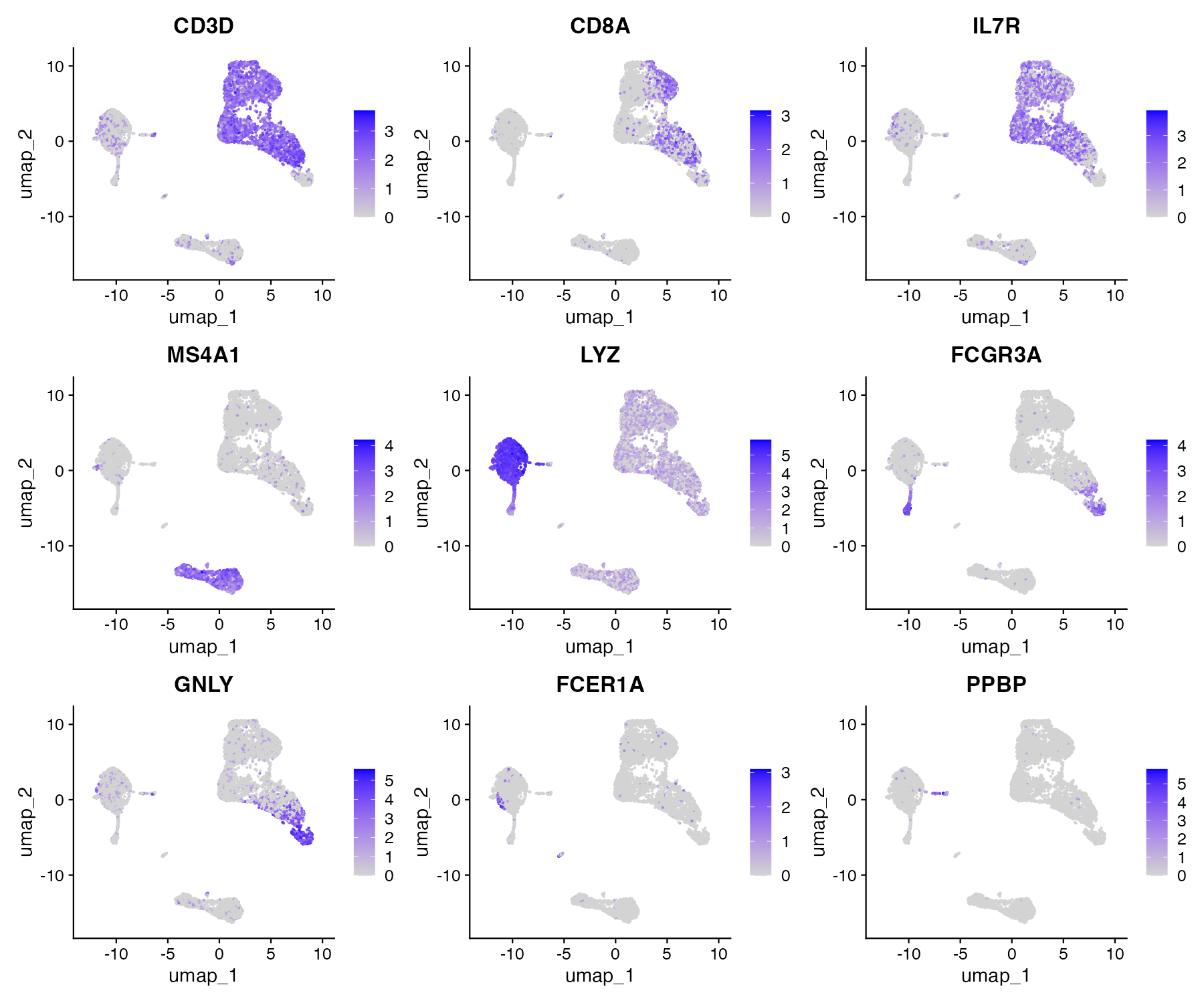
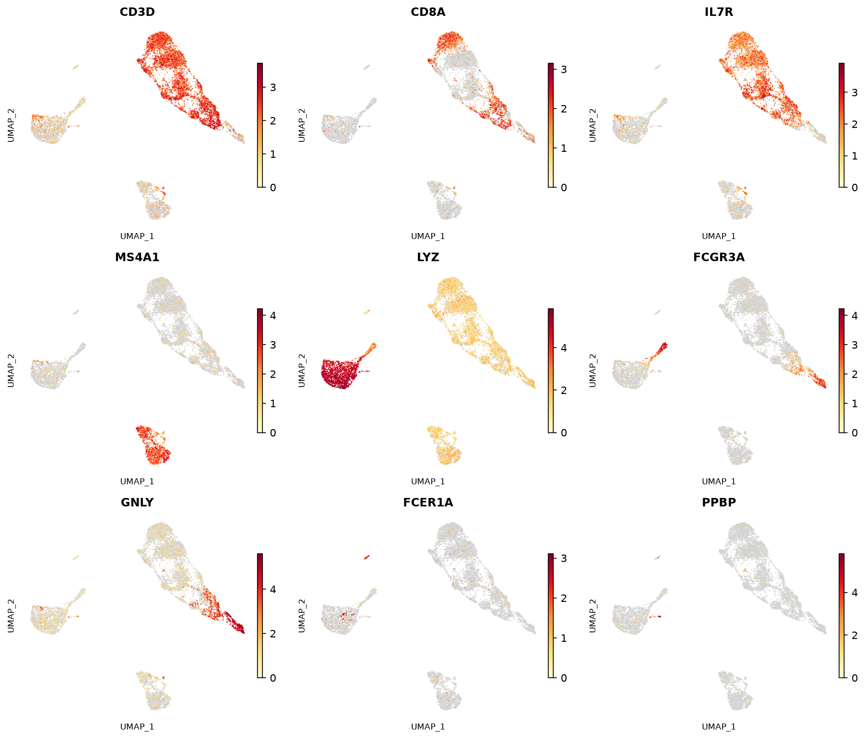
Canonical lineage markers identify the major PBMC populations. Truecell's annotate_clusters() helper z-scores each marker across clusters and assigns every cluster to its most-enriched lineage.

R (Seurat) Python (Truecell)

FeaturePlot(pbmc, c("CD3D","CD8A","IL7R","MS4A1",
                    "LYZ","FCGR3A","GNLY","FCER1A","PPBP"))

new.ids <- c("CD14+ Mono","CD4 T","CD8 T","CD4 T","CD8 T",
             "B","B","NK","CD4 T","FCGR3A+ Mono","DC","Platelet")
names(new.ids) <- levels(pbmc)
pbmc <- RenameIdents(pbmc, new.ids)
DimPlot(pbmc, label = TRUE)

from truecell.plotting import feature_plot
from tutorials.pbmc8k_subclustering_tutorial import annotate_clusters, BROAD_MARKERS

feature_plot(pbmc, ["CD3D","CD8A","IL7R","MS4A1",
                    "LYZ","FCGR3A","GNLY","FCER1A","PPBP"], ncol=3)

broad = annotate_clusters(pbmc, BROAD_MARKERS)
pbmc.stash_ident("global_clusters")
pbmc.rename_idents(broad)
dim_plot(pbmc, reduction="umap", label=True)

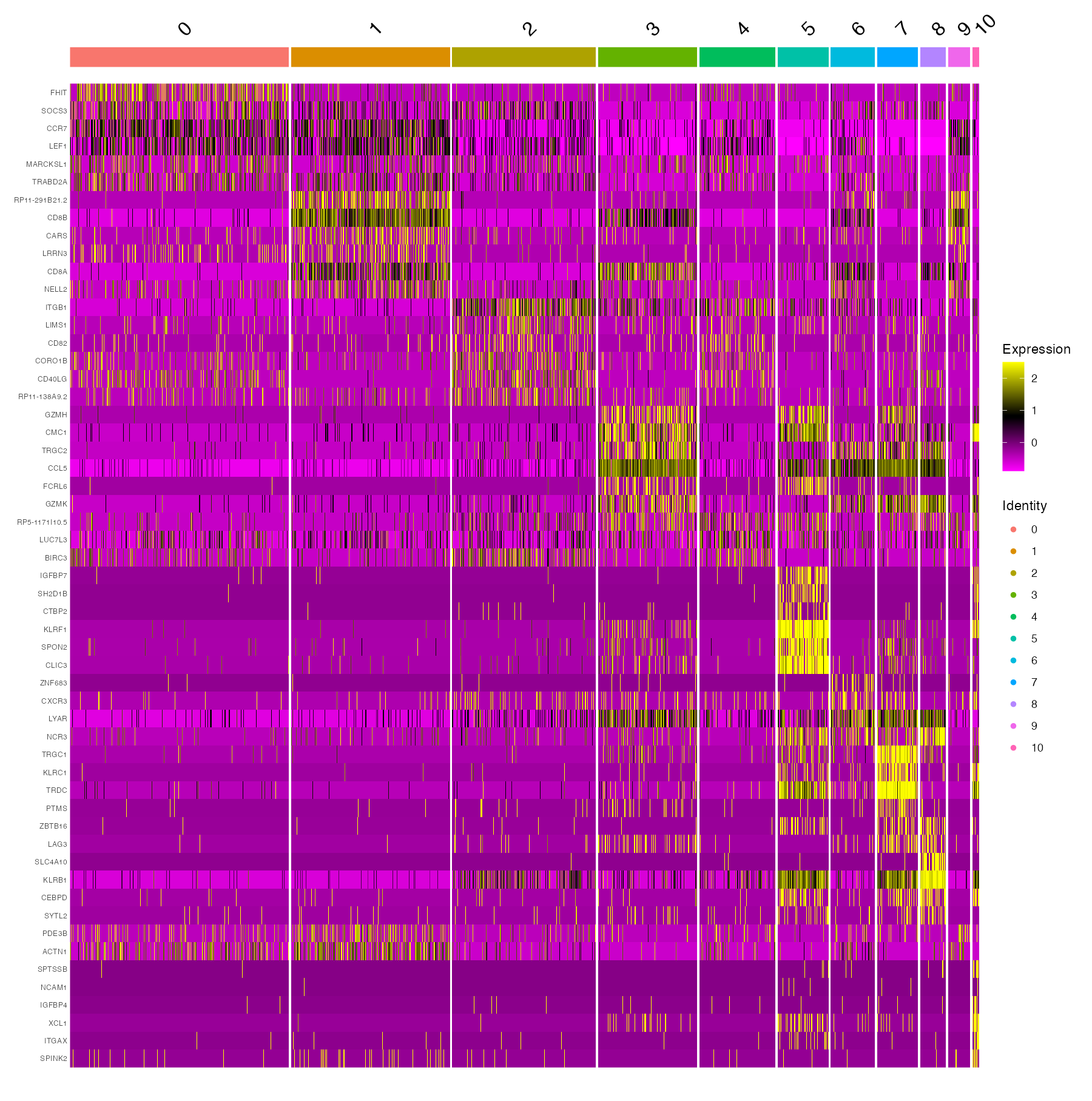
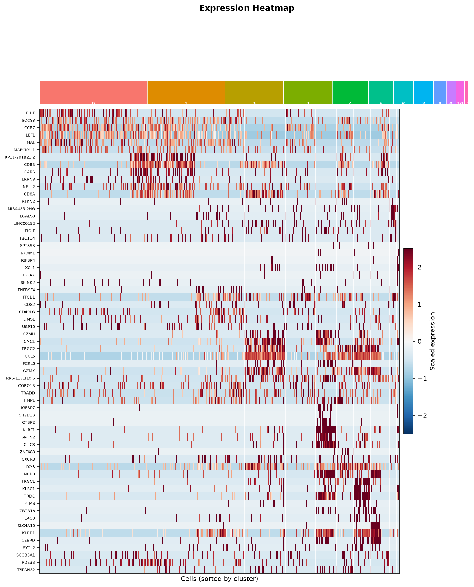
Top markers per cluster (DoHeatmap → do_heatmap):

R (Seurat)	Python (Truecell)

Step 6 · Subcluster the T/NK Compartment ⭐¶

This is the advanced step. The global clustering lumps several T-cell states together. We isolate the T/NK lineages and re-run the entire workflow on just those cells — recomputing variable genes, PCA, neighbours, clusters, and UMAP within the compartment. This is the standard Seurat subclustering recipe.

R (Seurat) Python (Truecell)

tnk <- subset(pbmc, idents = c("CD4 T","CD8 T","NK"))

tnk <- FindVariableFeatures(tnk, nfeatures = 2000)
tnk <- ScaleData(tnk, features = rownames(tnk))
tnk <- RunPCA(tnk, npcs = 30)
tnk <- FindNeighbors(tnk, dims = 1:10)
tnk <- FindClusters(tnk, resolution = 0.6)
tnk <- RunUMAP(tnk, dims = 1:10)
DimPlot(tnk, label = TRUE)

# cells in the T/NK lineages (from the broad annotation above)
gid = pbmc.meta_data["global_clusters"].astype(str).values
lymphoid = {c for c, lin in broad.items() if lin in {"CD4 T","CD8 T","NK"}}
tnk_cells = [c for c, g in zip(pbmc.cell_names(), gid) if g in lymphoid]

tnk = pbmc.subset(cells=tnk_cells)              # ~4,600 cells
# data layer already normalised → re-run from HVG onward
find_variable_features(tnk, selection_method="vst", nfeatures=2000)
scale_data(tnk, features=tnk.assays["RNA"]._all_feature_names)
run_pca(tnk, n_pcs=30, features=tnk.assays["RNA"].variable_features)
find_neighbors(tnk, dims=range(10), k_param=20)
find_clusters(tnk, resolution=0.6, random_seed=0)
run_umap(tnk, dims=range(10), seed=42)
dim_plot(tnk, reduction="umap", group_by="seurat_clusters", label=True)

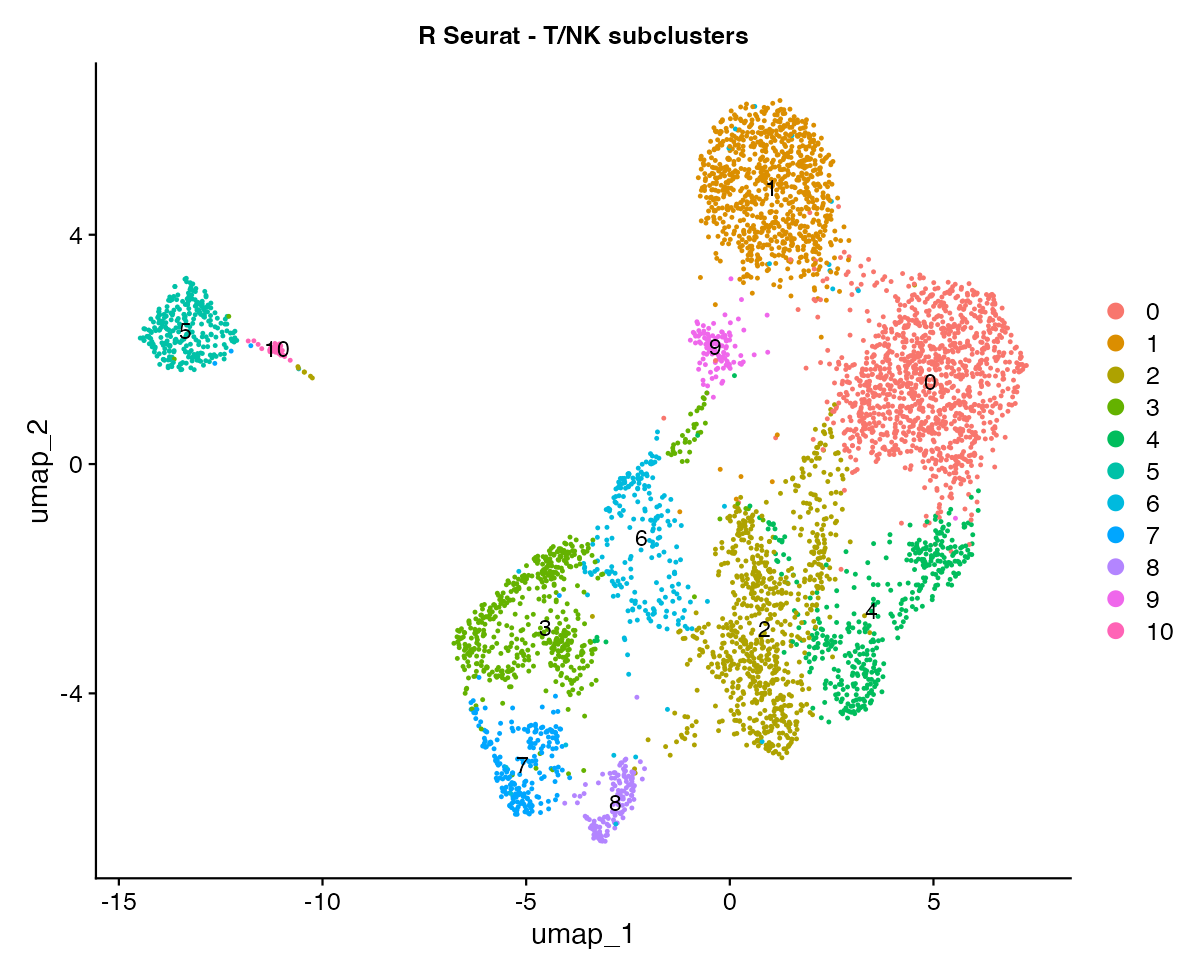
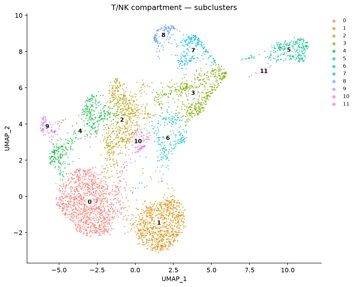
The whole pipeline is wrapped in run_pipeline() / run_full() in pbmc8k_subclustering_tutorial.py, so the subclustering is a single pbmc.subset(...) followed by the same calls.

Step 7 · Annotate the Fine T/NK Subsets¶

Flat marker-argmax fails for fine T subsets (the high-magnitude naive markers CCR7/SELL outscore the low-magnitude but definitive CD8B), so annotate_tnk_subsets() gates in lineage-priority order — NK (CD3⁻, NKG7/GNLY⁺) → CD8/cytotoxic T (CD8A/B or a CD3⁺ NKG7/GZMK program, which also captures MAIT/γδ T) → CD4 Naive (CCR7/SELL/LEF1) → CD4 Memory (IL7R/S100A4).

R (Seurat)	Python (Truecell)
`FeaturePlot(tnk, c("CCR7","SELL","IL7R","S100A4", "CD8A","GZMK","GNLY","NKG7")) VlnPlot(tnk, c("CCR7","S100A4","CD8A","GNLY")) # manual annotation by canonical markers tnk <- RenameIdents(tnk, sub.ids) DimPlot(tnk, label = TRUE)`	`from tutorials.pbmc8k_subclustering_tutorial import annotate_tnk_subsets feature_plot(tnk, ["CCR7","SELL","IL7R","S100A4", "CD8A","GZMK","GNLY","NKG7"], ncol=4) vln_plot(tnk, ["CCR7","S100A4","CD8A","GNLY"], ncol=2) sub_anno = annotate_tnk_subsets(tnk) tnk.stash_ident("sub_clusters") tnk.rename_idents(sub_anno) dim_plot(tnk, reduction="umap", label=True)`

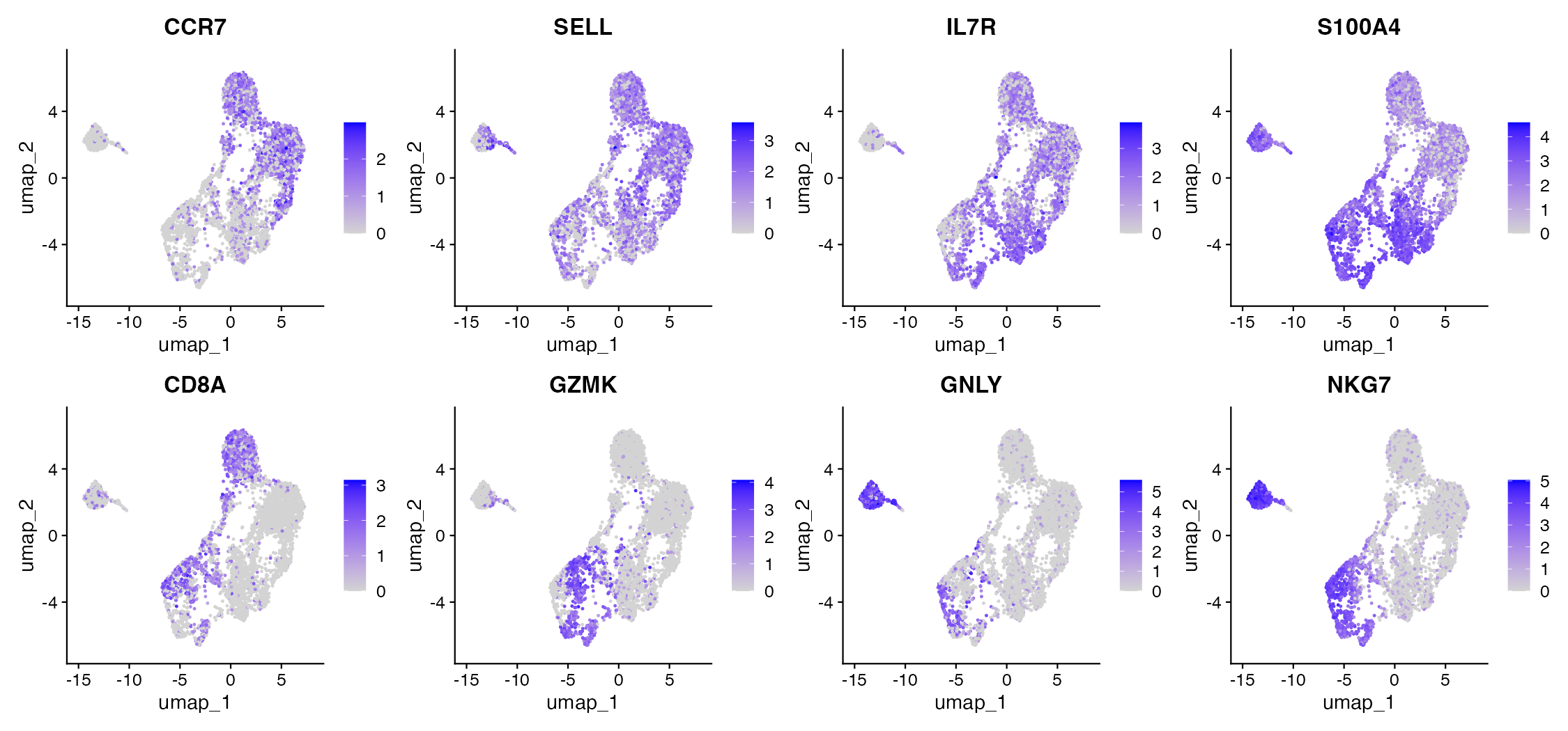
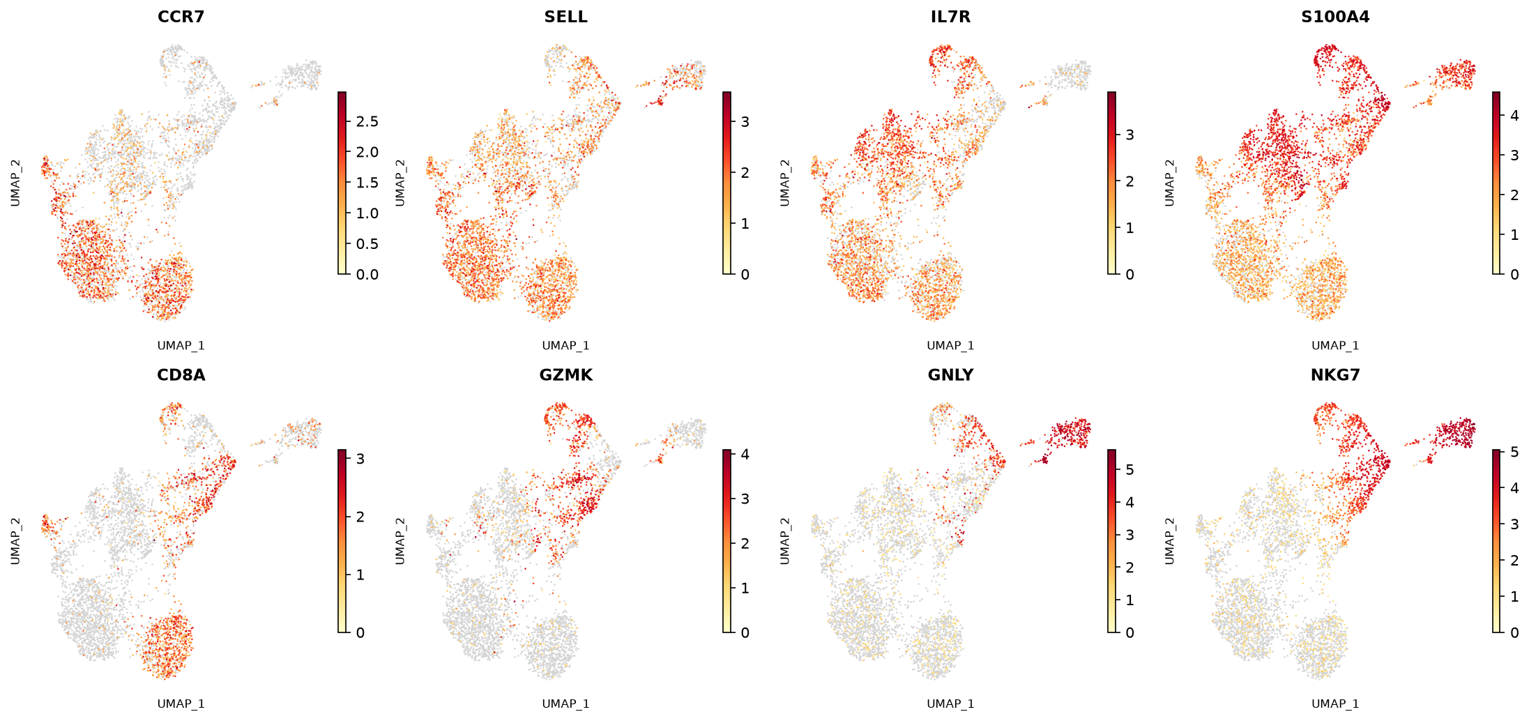
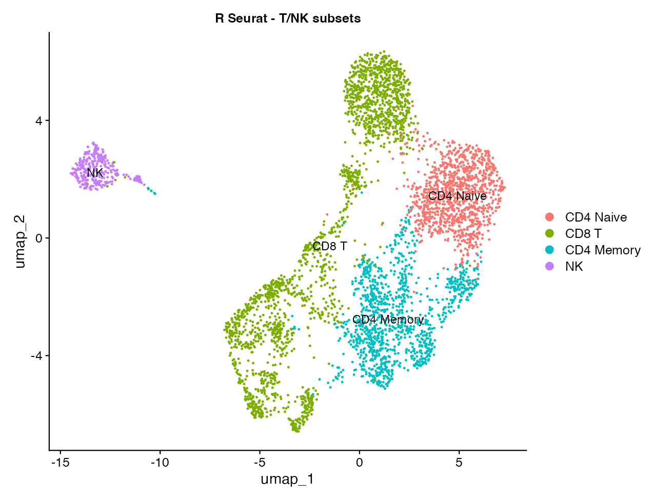
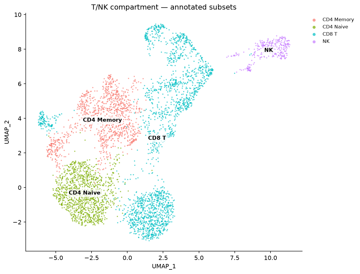
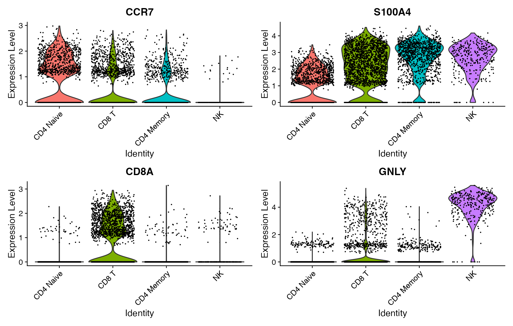
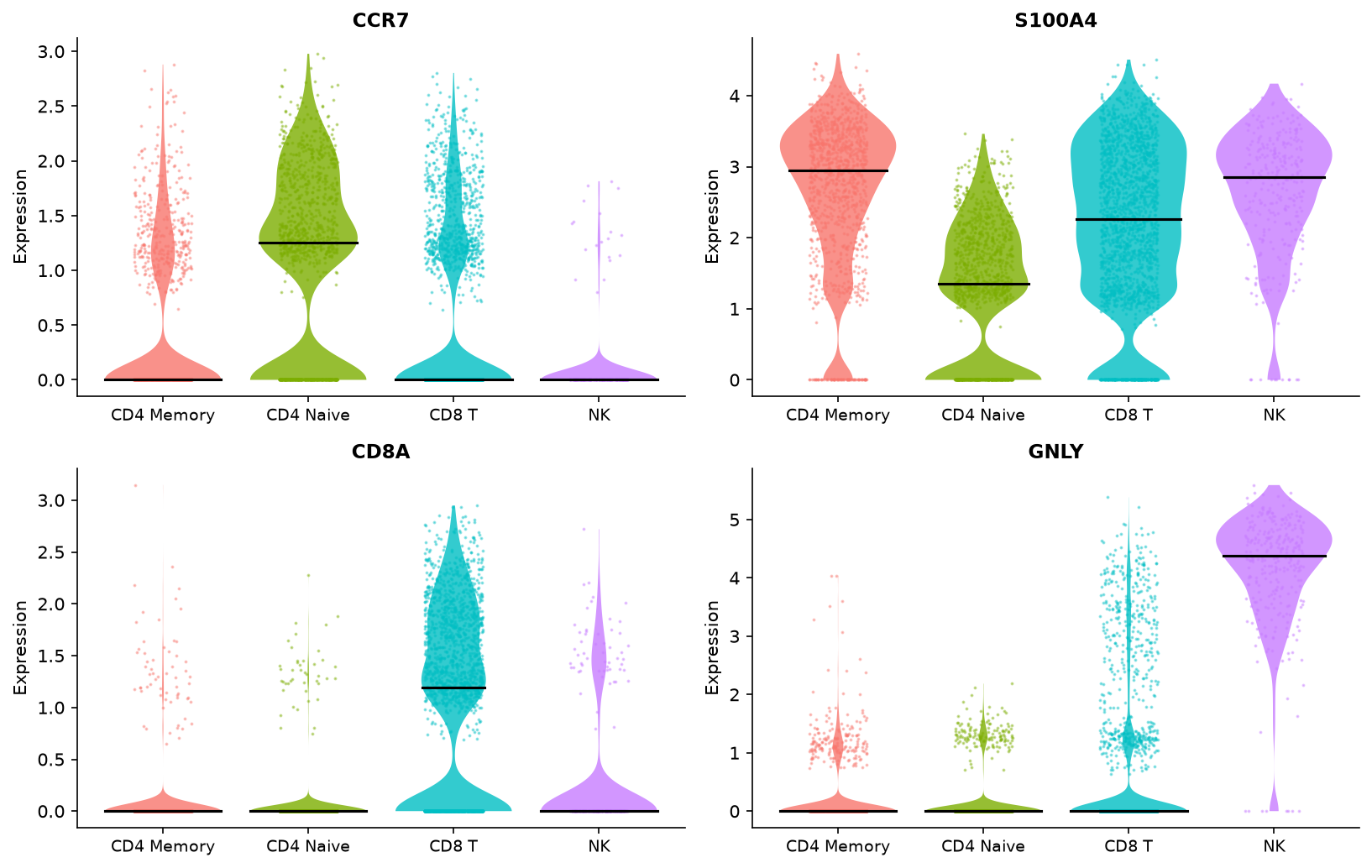
What the subclustering reveals¶

Substructure that the 12 global clusters did not separate:

Subset	Defining markers	Notes
CD4 Naive	`CCR7`, `SELL`, `LEF1` (+ ribosomal)	quiescent helper T
CD4 Memory	`IL7R`, `S100A4`, `LTB`	activated/memory helper T
CD8 T	`CD8A`, `CD8B`, `GZMK`, `CCL5`	naive + cytotoxic effector
NK	`GNLY`, `NKG7`, `KLRD1`, `PRF1`	CD3-negative cytotoxic

The CD8/cytotoxic group also resolves a TRDC/TRGC1 γδ-T subcluster and a KLRB1/NCR3 MAIT subcluster — unconventional cytotoxic T cells that are invisible at the global resolution.

How close is this to Seurat?¶

Every figure above is a side-by-side, which means it was checked by eye. pbmc8k_subclustering_verify.R also writes a numeric handoff, and --report compares it:

python tutorials/pbmc8k_subclustering_tutorial.py          # writes the Python side
Rscript tutorials/pbmc8k_subclustering_verify.R            # writes the R side
python tutorials/pbmc8k_subclustering_tutorial.py --report

Nothing is pinned across the two sides. Both run the whole two-stage pipeline from the same 10x bytes.

Stage	truecell vs Seurat 5.5.1
QC	the same 7,475 barcodes; nCount and nFeature exact, percent.mt to 5.3e-15
Normalized data	total to 8.2e-13 relative · kNN graph 149,500 on both
Stage 1 clusters	13 vs 12 · ARI 0.977 · 7,341/7,475 cells agree
Broad lineage, per cell	0.9858
T/NK compartment	Jaccard 0.9991 — 4,631 of 4,635 cells are the same barcodes
Stage 2 subclusters	12 vs 11 · ARI 0.916 on the shared cells
T/NK subset label, per cell	0.9821; the four subset sizes agree within 25 cells

Why the compartment is compared by barcode¶

The T/NK compartment is the number to watch, and it is the reason the handoff dumps cell tables rather than summary counts. Everything in stage two is conditioned on which cells stage one selected — so a subclustering fed from the wrong global clusters would still produce a compartment of a plausible size, still produce subclusters, still produce a marker table, and a size check would call all of it a match. Only comparing the barcodes can tell "the same 4,600 cells" from "4,600 cells". Here they are the same to four cells.

The extra cluster¶

truecell finds 13 global clusters where Seurat finds 12. Seurat's 100-cell cluster 11 holds both Platelet and DC; truecell splits it into a 54-cell DC cluster and a 53-cell Platelet cluster. Two distinct myeloid lineages, so the split is the more resolved answer.

Note that this runs opposite to the PBMC 3k tutorial, where Seurat resolves a 32-cell DC cluster that truecell folds into CD14+ Mono. Both are the same borderline population landing on different sides of a resolution threshold, and neither run is uniformly finer than the other — which is worth knowing before reading a cluster count as a verdict.

API Translation (additions beyond the PBMC 3k tutorial)¶

Task	R (Seurat)	Python (Truecell)
Load PBMC 8k	`Read10X("…/GRCh38/")`	`pbmc8k()`
Subset a lineage	`subset(pbmc, idents = …)`	`pbmc.subset(cells = …)`
Stash current ids	`pbmc$old <- Idents(pbmc)`	`pbmc.stash_ident("old")`
Re-cluster subset	re-run `FindVariableFeatures…FindClusters`	re-run `find_variable_features…find_clusters`

References¶

Satija R, Farrell JA, Gennert D, Schier AF, Regev A (2015). Spatial reconstruction of single-cell gene expression data. Nature Biotechnology 33, 495–502. https://doi.org/10.1038/nbt.3192

Butler A, Hoffman P, Smibert P, Papalexi E, Satija R (2018). Integrating single-cell transcriptomic data across different conditions, technologies, and species. Nature Biotechnology 36, 411–420. https://doi.org/10.1038/nbt.4096

Hao Y, Hao S, Andersen-Nissen E, et al. (2021). Integrated analysis of multimodal single-cell data. Cell 184, 3573–3587. https://doi.org/10.1016/j.cell.2021.04.048

10x Genomics (2017). 8k PBMCs from a Healthy Donor. https://www.10xgenomics.com/datasets/8-k-pbm-cs-from-a-healthy-donor-2-standard-2-1-0