Multimodal Tutorial — CITE-seq (RNA + Protein) with R Seurat vs Truecell¶

A Python port of Seurat's multimodal vignette using the CBMC CITE-seq dataset (GSE100866): ~8,600 cord-blood mononuclear cells profiled simultaneously for the transcriptome and 13 surface proteins (antibody-derived tags, "ADT"). It showcases Truecell's multi-assay support: cluster on RNA, attach the protein counts as a second assay, CLR-normalise them, and read protein levels on the RNA-derived UMAP.

Dataset: 8k CBMCs, CITE-seq — Stoeckius et al. 2017 (GSE100866) Python: Truecell

Scope note. Truecell stores and normalises multiple assays, visualises one against another, and performs multimodal integration via Weighted Nearest Neighbor (WNN) analysis (Step 8) — learning a per-cell RNA-vs-protein weight and clustering both modalities jointly.

python tutorials/cbmc_citeseq_tutorial.py     # printed validation + the numeric handoff
python tutorials/generate_multimodal_plots.py # writes figures_multimodal/  (Truecell figures)
Rscript tutorials/cbmc_citeseq_verify.R       # R figures + r_adt_clr.csv / r_cell_weights.csv
python tutorials/cbmc_citeseq_tutorial.py --report   # the side-by-side, per protein and per cell

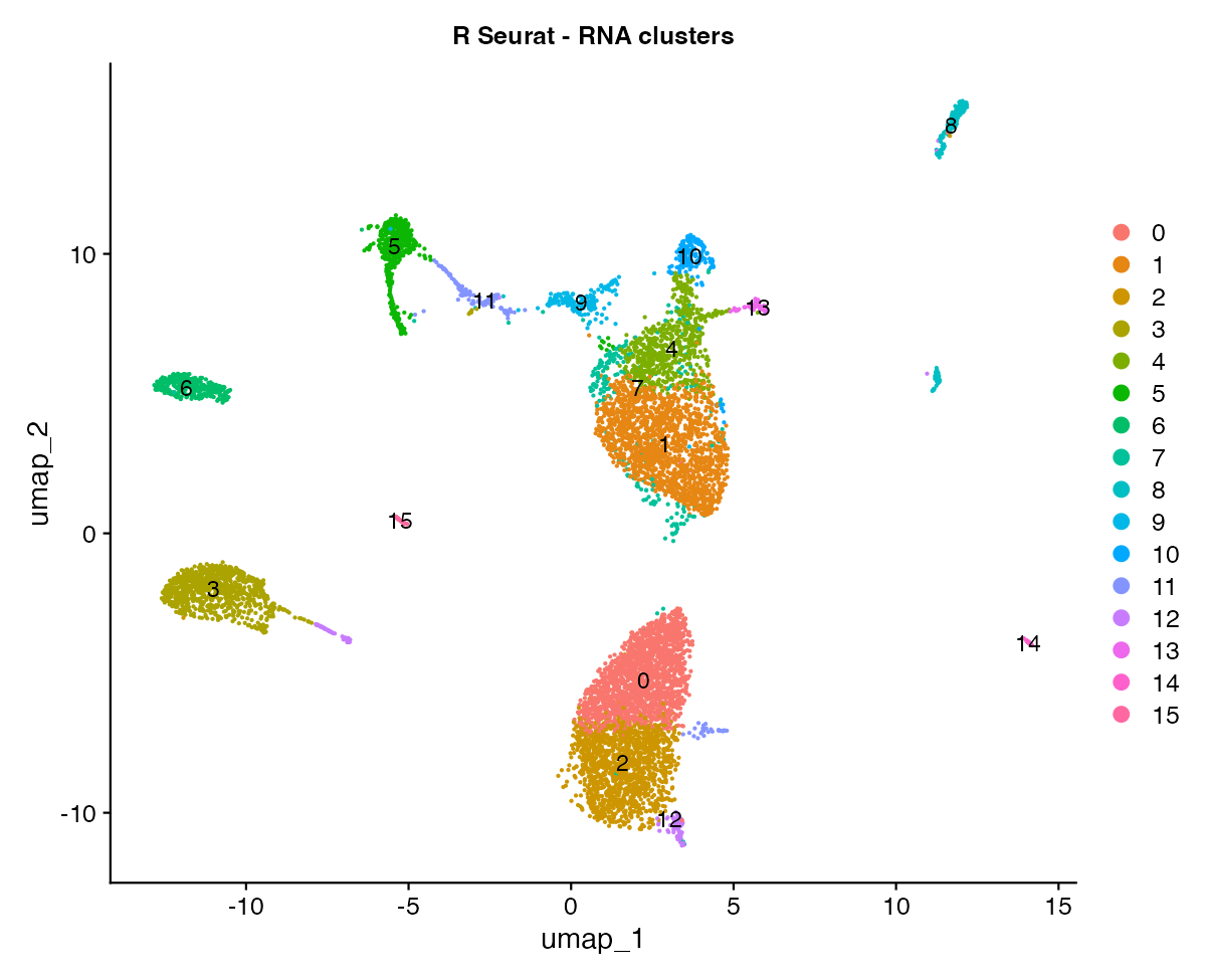
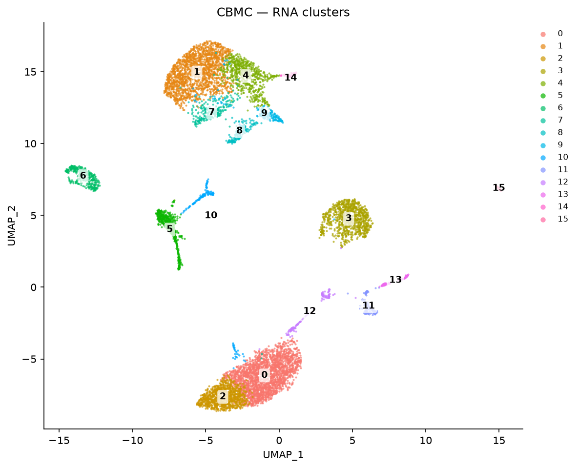
About the figures. Each step shows a genuine side-by-side comparison: the left image is real R Seurat output (cbmc_citeseq_verify.R, titled "R Seurat – …") and the right image is Truecell (generate_multimodal_plots.py). Both run the identical RNA workflow, the same CLR transform, and the same protein-gated annotation — with the same thresholds — on the same data, and both cluster with Seurat's modularity optimiser. The neighbour graphs they build still differ slightly, so compare the structure, not exact positions or cluster numbers.

Step 1 · Load RNA + Protein, align barcodes¶

The RNA matrix mixes human and mouse spike-in genes; both Seurat and Truecell keep the human genes. RNA and ADT are aligned to their shared cell barcodes.

R (Seurat) Python (Truecell)

library(Seurat)
cbmc.rna <- as.sparse(read.csv("GSE100866_...RNA_umi.csv.gz", row.names = 1))
cbmc.rna <- CollapseSpeciesExpressionMatrix(cbmc.rna)   # keep human
cbmc.adt <- as.sparse(read.csv("GSE100866_...ADT_umi.csv.gz", row.names = 1))

joint <- intersect(colnames(cbmc.rna), colnames(cbmc.adt))
cbmc.rna <- cbmc.rna[, joint]
cbmc.adt <- cbmc.adt[, joint]

from truecell.datasets import cbmc_citeseq
# downloads ~15 MB, keeps human genes, aligns shared barcodes
rna, genes, adt, proteins, cells = cbmc_citeseq()
# rna: (20379 genes x 8617 cells)   adt: (13 proteins x 8617 cells)
# proteins: CD3 CD4 CD8 CD45RA CD56 CD16 CD10 CD11c CD14 CD19 CD34 CCR5 CCR7

Step 2 · Create the object & run the RNA workflow¶

R (Seurat) Python (Truecell)

cbmc <- CreateSeuratObject(counts = cbmc.rna)
cbmc <- NormalizeData(cbmc)
cbmc <- FindVariableFeatures(cbmc)
cbmc <- ScaleData(cbmc)
cbmc <- RunPCA(cbmc, npcs = 30)
cbmc <- FindNeighbors(cbmc, dims = 1:15)
cbmc <- FindClusters(cbmc, resolution = 0.6)
cbmc <- RunUMAP(cbmc, dims = 1:15)

from truecell.truecell import create_truecell_object
from truecell.preprocessing import normalize_data, find_variable_features, scale_data
from truecell.reduction import run_pca
from truecell.neighbors import find_neighbors
from truecell.clustering import find_clusters
from truecell.umap import run_umap

obj = create_truecell_object(counts=rna, assay="RNA", min_cells=3,
                           feature_names=genes, cell_names=cells, project="cbmc")
normalize_data(obj)
find_variable_features(obj, selection_method="vst", nfeatures=2000)
scale_data(obj, features=obj.assays["RNA"]._all_feature_names)
run_pca(obj, n_pcs=30, features=obj.assays["RNA"].variable_features)
find_neighbors(obj, dims=range(15), k_param=20)
find_clusters(obj, resolution=0.6, random_seed=0)
run_umap(obj, dims=range(15), seed=42)

Step 3 · Add the protein (ADT) assay & CLR-normalise¶

The antibody counts become a second assay. Proteins are normalised with the centered-log-ratio transform, applied per cell across the 13-protein panel (margin = 2) — the recommended setting for small ADT panels.

R (Seurat) Python (Truecell)

adt_assay <- CreateAssayObject(counts = cbmc.adt)
cbmc[["ADT"]] <- adt_assay

cbmc <- NormalizeData(cbmc, assay = "ADT",
                      normalization.method = "CLR", margin = 2)

from truecell.assay5 import create_assay5_object

obj.assays["ADT"] = create_assay5_object(
    counts=adt_aligned, feature_names=proteins,
    cell_names=obj.cell_names(), key="adt_",
)
normalize_data(obj, assay="ADT", normalization_method="CLR", margin=2)
# obj.assay_names() -> ['RNA', 'ADT']

margin means exactly what it means in Seurat, axis included: Seurat's CustomNormalize runs apply(data, MARGIN = margin, clr_function), and R's apply treats MARGIN = 1 as rows and MARGIN = 2 as columns. So with counts stored features × cells, margin = 1 normalises each protein across cells (Seurat's default) and margin = 2 normalises each cell across its proteins (what ADT panels want). Truecell had these two swapped until the fix described at the end of Step 8.

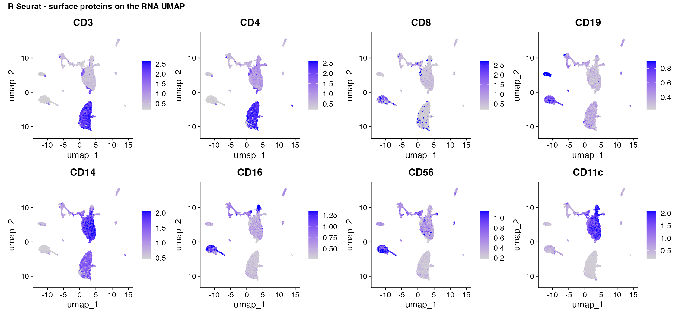
Step 4 · Visualise protein on the RNA UMAP¶

In R you switch DefaultAssay() (or use the adt_/rna_ key prefixes); in Truecell you pass assay="ADT".

R (Seurat) Python (Truecell)

DefaultAssay(cbmc) <- "ADT"
FeaturePlot(cbmc, c("CD3","CD4","CD8","CD19",
                    "CD14","CD16","CD56","CD11c"))

from truecell.plotting import feature_plot

feature_plot(obj, ["CD3","CD4","CD8","CD19",
                   "CD14","CD16","CD56","CD11c"],
             assay="ADT", reduction="umap",
             min_cutoff="q05", max_cutoff="q95", ncol=4)

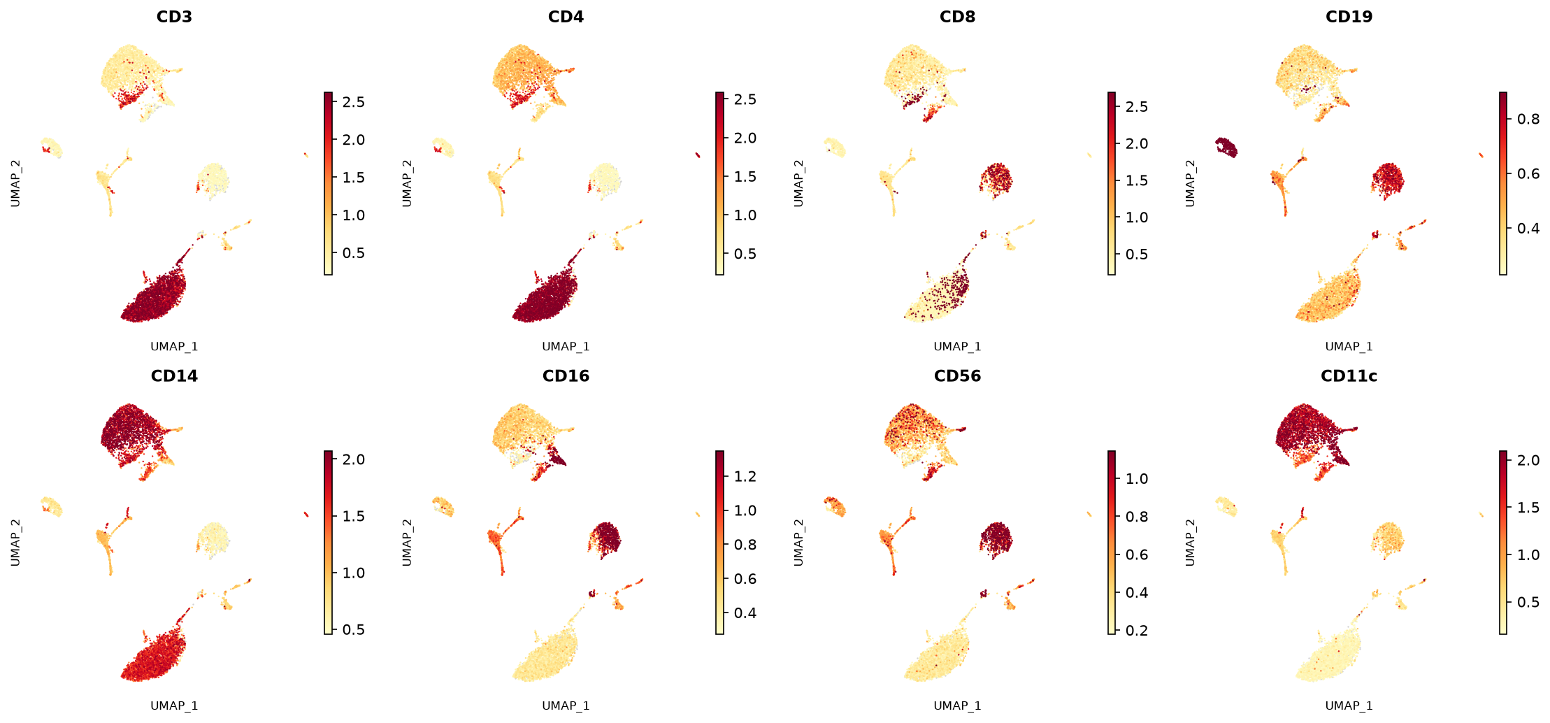The surface proteins cleanly mark their lineages: CD3/CD4 the T-cell mass, CD19 the B-cell island, CD8/CD16/CD56 the NK cluster, CD14/CD11c the monocytes.

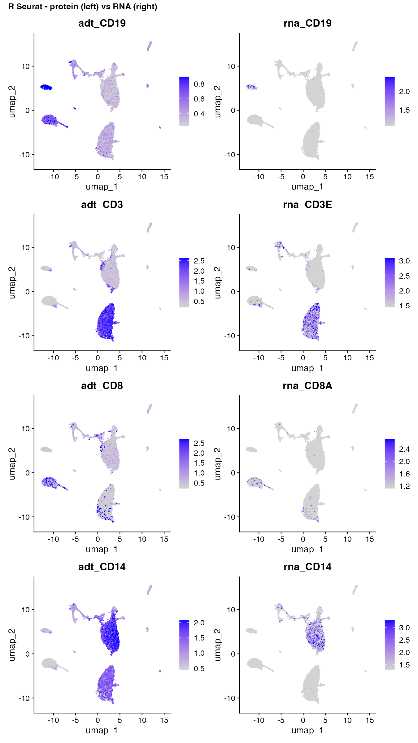
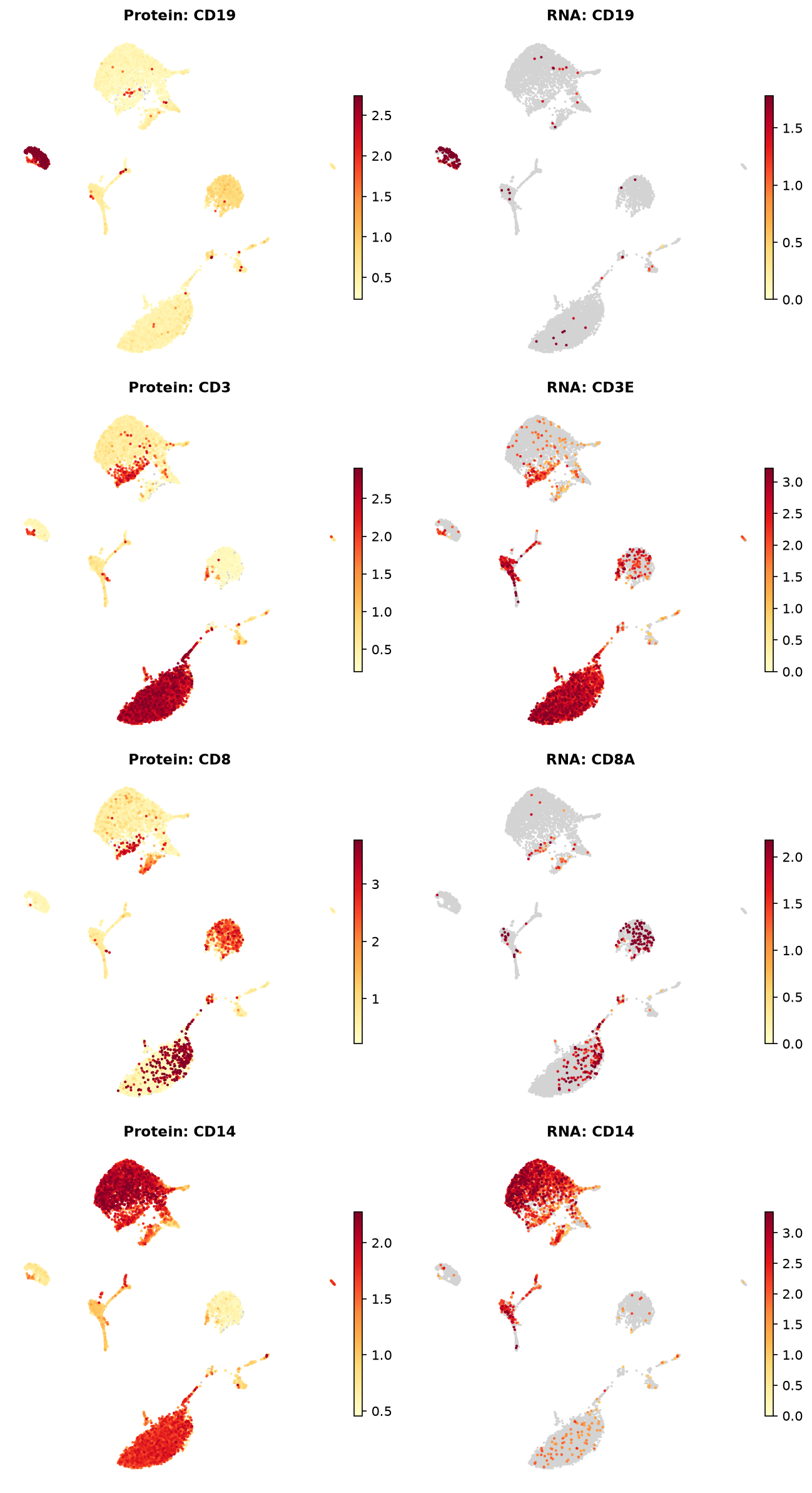
Step 5 · Protein vs RNA for the same marker¶

The CITE-seq payoff: protein gives a smooth, high signal-to-noise readout where the encoding mRNA is sparse and noisy.

R (Seurat) Python (Truecell)

# adt_ / rna_ key prefixes pull from each assay
FeaturePlot(cbmc, c("adt_CD19", "rna_CD19",
                    "adt_CD3",  "rna_CD3E"), ncol = 2)

# left column assay="ADT", right column assay="RNA"
feature_plot(obj, ["CD19"], assay="ADT", reduction="umap")
feature_plot(obj, ["CD19"], assay="RNA", reduction="umap")
# (generate_multimodal_plots.py draws them paired)

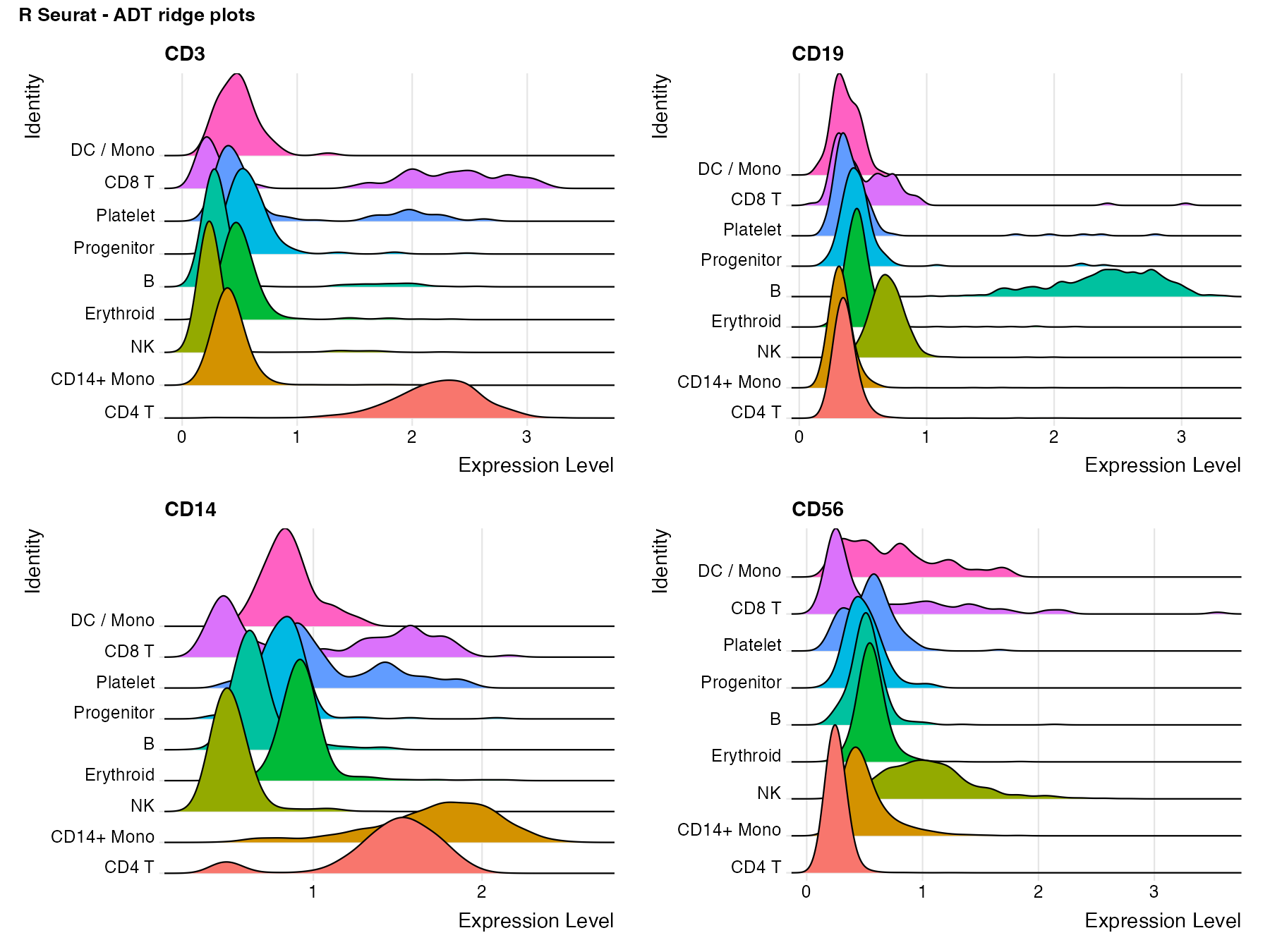
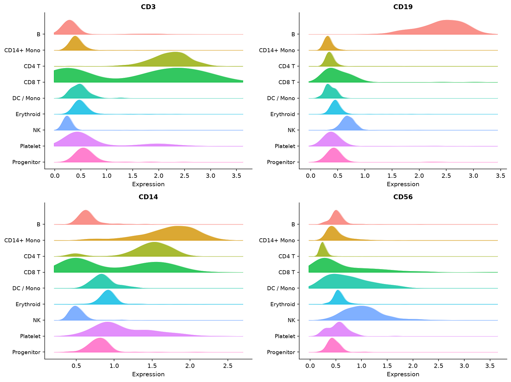
Step 6 · Ridge plots & protein bivariates¶

R (Seurat)	Python (Truecell)
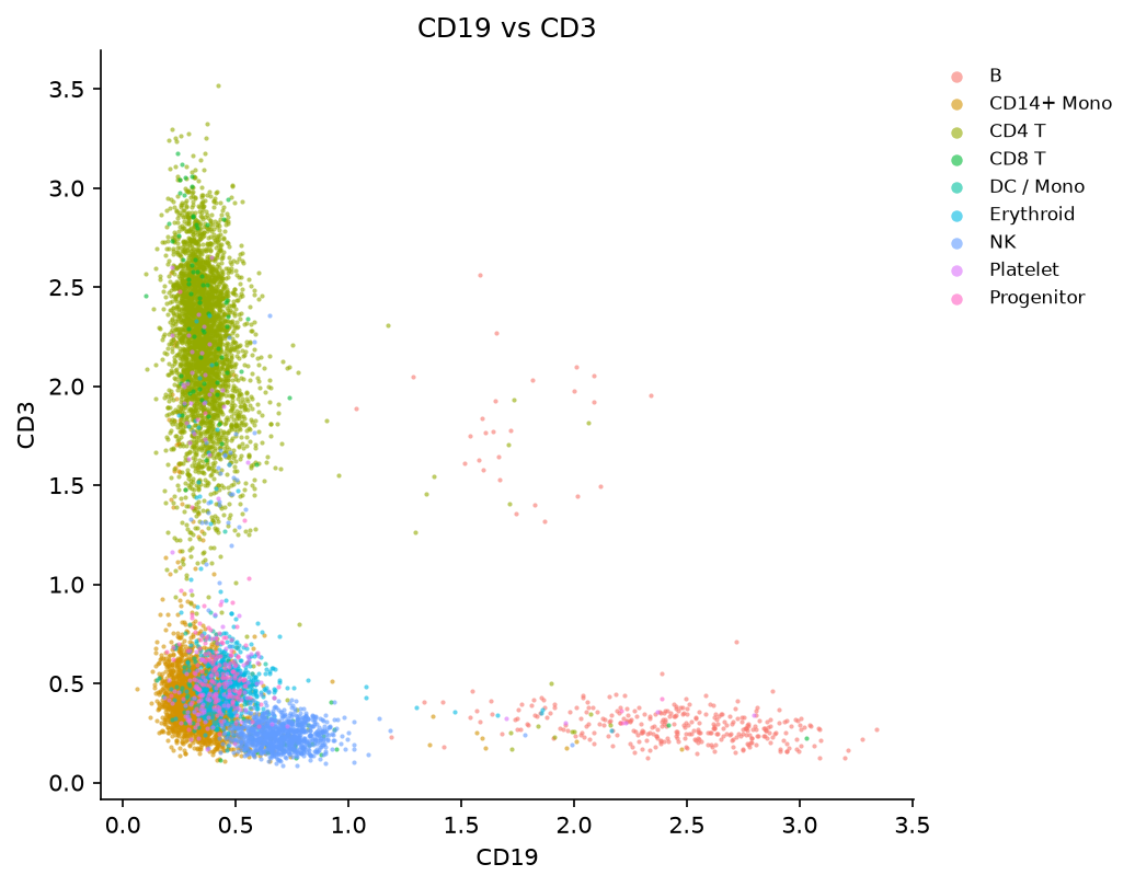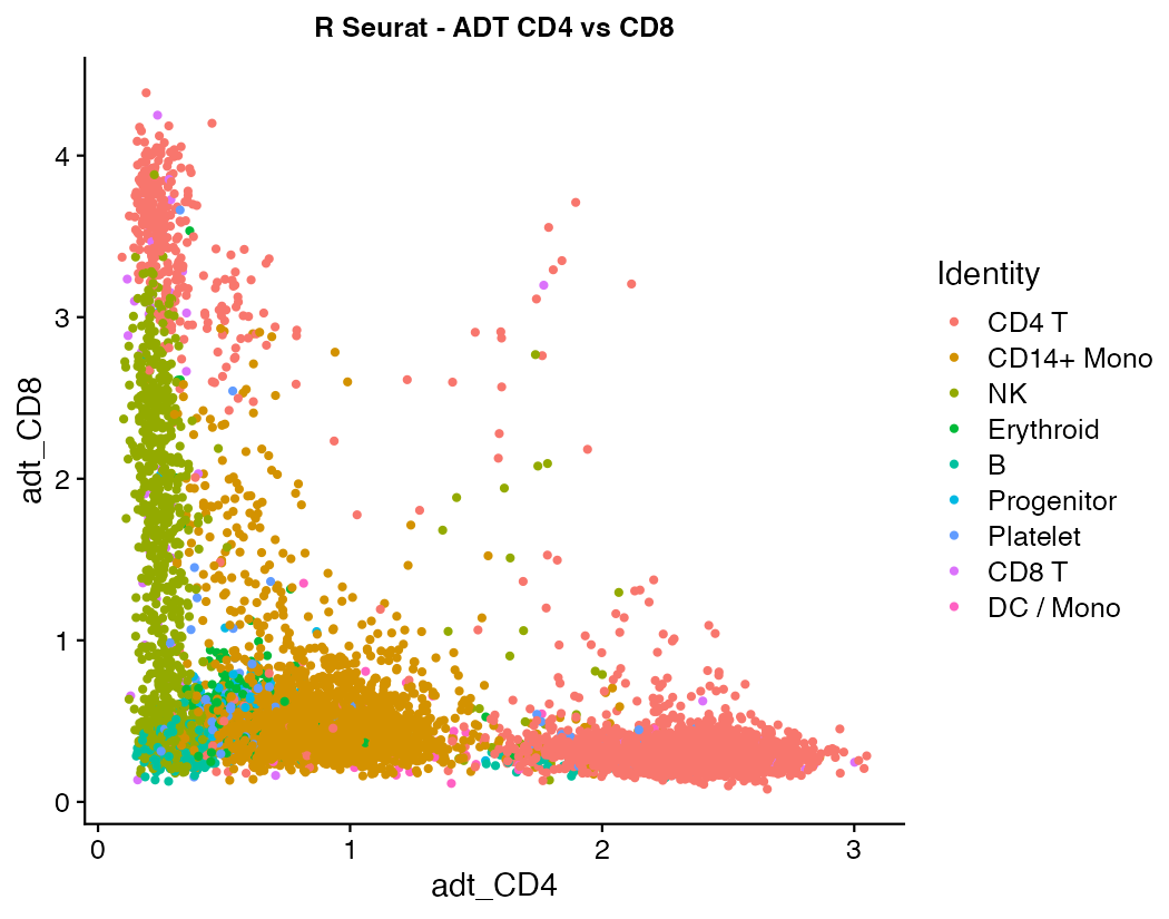
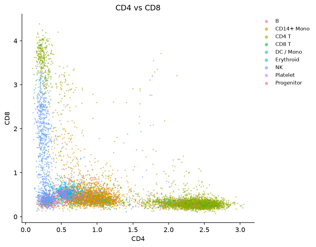
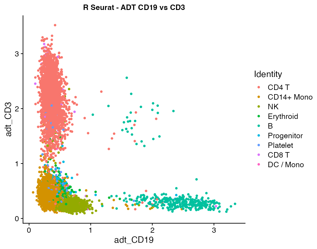
`RidgePlot(cbmc, features = c("adt_CD3","adt_CD19", "adt_CD14","adt_CD56"), ncol = 2) FeatureScatter(cbmc, "adt_CD19", "adt_CD3") FeatureScatter(cbmc, "adt_CD4", "adt_CD8")`	`from truecell.plotting import ridge_plot, feature_scatter ridge_plot(obj, ["CD3","CD19","CD14","CD56"], assay="ADT", group_by="protein_celltype", ncol=2) feature_scatter(obj, "CD19", "CD3", assay="ADT") feature_scatter(obj, "CD4", "CD8", assay="ADT")`

The CD4-vs-CD8 and CD19-vs-CD3 protein scatters separate the major lineages on just two axes.

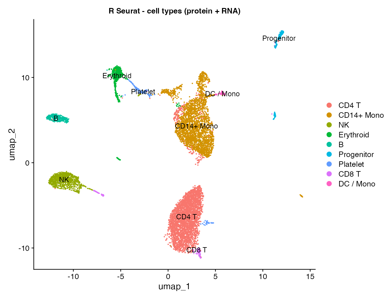
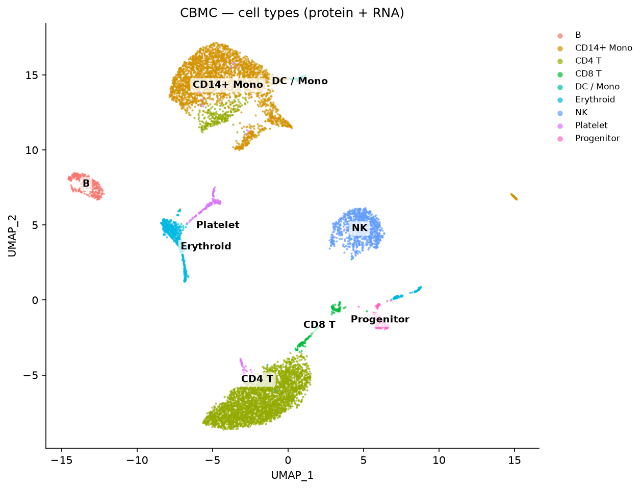
Step 7 · Annotate cell types (protein + RNA)¶

CITE-seq proteins are cleaner lineage markers than RNA, so annotate_cells() gates on the ADT assay (T→NK→B→monocyte→DC→progenitor) and falls back to RNA markers for populations the 13-protein panel can't resolve — platelets (PPBP), erythroid (HBB), pDC (IGJ/PLD4), and cycling cells.

R (Seurat) Python (Truecell)

# manual, by inspecting protein + RNA markers
cbmc <- RenameIdents(cbmc, ...)
DimPlot(cbmc, label = TRUE)

from tutorials.cbmc_citeseq_tutorial import annotate_cells
from truecell.plotting import dim_plot

anno = annotate_cells(obj)
obj.stash_ident("rna_clusters")
obj.rename_idents(anno)
dim_plot(obj, reduction="umap", group_by="protein_celltype", label=True)

Step 8 · Weighted Nearest Neighbor (WNN) multimodal clustering¶

Steps 2–7 cluster on RNA alone and read protein on top. WNN (Hao et al., Cell 2021) goes further: it learns, per cell, how much to trust each modality and clusters on a joint graph. A cell whose lineage is crisp in protein space is weighted toward ADT; a cell the antibody panel can say nothing useful about is weighted toward RNA.

Crucially the weights are decisive, not hedged: they use the full 0–1 range, and most cells commit to one modality rather than sitting at 0.5. That is by design — the modality score is clipped at 200 before the softmax, so a cell with a clear preference saturates.

Which cells end up on which side is an empirical result, not something you can read off the panel design. Mostly the table below tracks the panel, but not everywhere: CD8 T leans on RNA (0.37) even though CD8 is one of the 13 antibodies, while CD4 T leans the other way at 0.64. Seurat says the same (0.38 / 0.64), so it is a property of the data and the method rather than of this port — but this tutorial does not explain it.

The protein modality first gets its own reduction ("apca"); then find_multi_modal_neighbors builds the joint wknn/wsnn graphs and writes a per-cell weight for each modality. Clustering and UMAP then run on the joint graph instead of the RNA PCA.

R (Seurat) Python (Truecell)

DefaultAssay(cbmc) <- "ADT"
VariableFeatures(cbmc) <- rownames(cbmc[["ADT"]])
cbmc <- ScaleData(cbmc)
# 13 proteins, so npcs must stay well under that; irlba needs
# the gap, hence approx = FALSE
cbmc <- RunPCA(cbmc, reduction.name = "apca", reduction.key = "apca_",
               npcs = 12, approx = FALSE)

cbmc <- FindMultiModalNeighbors(
  cbmc, reduction.list = list("pca", "apca"),
  dims.list = list(1:15, 1:12), k.nn = 20
)
cbmc <- FindClusters(cbmc, graph.name = "wsnn", resolution = 0.6)
cbmc <- RunUMAP(cbmc, nn.name = "weighted.nn",
                reduction.name = "wnn.umap")

# per-cell modality weights land in metadata:
#   cbmc$RNA.weight , cbmc$ADT.weight

from truecell.reduction import run_pca
from truecell.preprocessing import scale_data
from truecell.multimodal import find_multi_modal_neighbors

# protein modality needs its own reduction
adt_features = obj.assays["ADT"]._all_feature_names
scale_data(obj, assay="ADT", features=adt_features)
run_pca(obj, assay="ADT", reduction_name="apca",
        reduction_key="apca_", n_pcs=12, features=adt_features)

find_multi_modal_neighbors(
    obj, reduction_list=["pca", "apca"],
    dims_list=[range(15), range(12)], k_nn=20,
)
find_clusters(obj, graph_name="wsnn", resolution=0.6, random_seed=0)
run_umap(obj, graph="wsnn", reduction_name="wnn_umap", seed=42)

# per-cell modality weights land in meta_data:
#   obj.meta_data["RNA.weight"] , obj.meta_data["ADT.weight"]

Because the ADT panel has only 13 proteins, apca keeps every informative component (n_pcs ≤ 12). Inspect the learned weights by grouping ADT.weight by the Step-7 labels:

obj.meta_data.groupby("protein_celltype")["ADT.weight"].mean().sort_values(ascending=False)

The lineages the antibody panel targets head-on lean on protein, and the ordering tracks how well the panel covers each type. Seurat's numbers on the same data are alongside:

Cell type	Truecell `ADT.weight`	R Seurat	in the panel?
NK	0.65	0.65	CD16 + CD56
CD4 T	0.64	0.64	CD4 — and CD4/CD8 is a protein call, not an RNA one
B	0.54	0.54	CD19
CD14+ Mono	0.48	0.49	CD14
Erythroid	0.40	0.40	✗
CD8 T	0.37	0.38	CD8
Platelet	0.29	0.30	✗
Progenitor	0.28	0.29	CD34 only
DC / Mono	—	0.21	✗ — no clean DC probe

The panel's targets sit at the top and the populations it cannot see sit at the bottom, which is the result you would hope for. DC / Mono is the case worth dwelling on: protein tells WNN almost nothing about those cells, so nearly all the weight goes to RNA. A weighting pinned near 0.5 could never express that. truecell's RNA clusters fold those 69 cells into CD14+ Mono, so the label gets no row of its own here, but truecell weights the same cells 0.21 as well. Erythroid and platelet carry no antibody either, and both duly fall back toward RNA.

Progenitor is the one row that does not line up — 0.35 here against R's 0.29, where every other type agrees to 0.02. It is a 146-cell population, and the two sides do not cut quite the same cells into it (R's progenitor cluster carries mean CD34 1.31, Truecell's 1.5).

This used to be as far as the tutorial could go: it read like small-population clustering noise rather than a difference in the WNN maths, but that was a reading. It is now established. Re-grouping Truecell's own per-cell weights by R's labels puts progenitor at 0.283 against R's 0.285 — the weights agree to three decimals, and the gap was entirely in which cells carry the label. See How close is this to Seurat? for the per-cell comparison that shows it.

Reading the plots¶

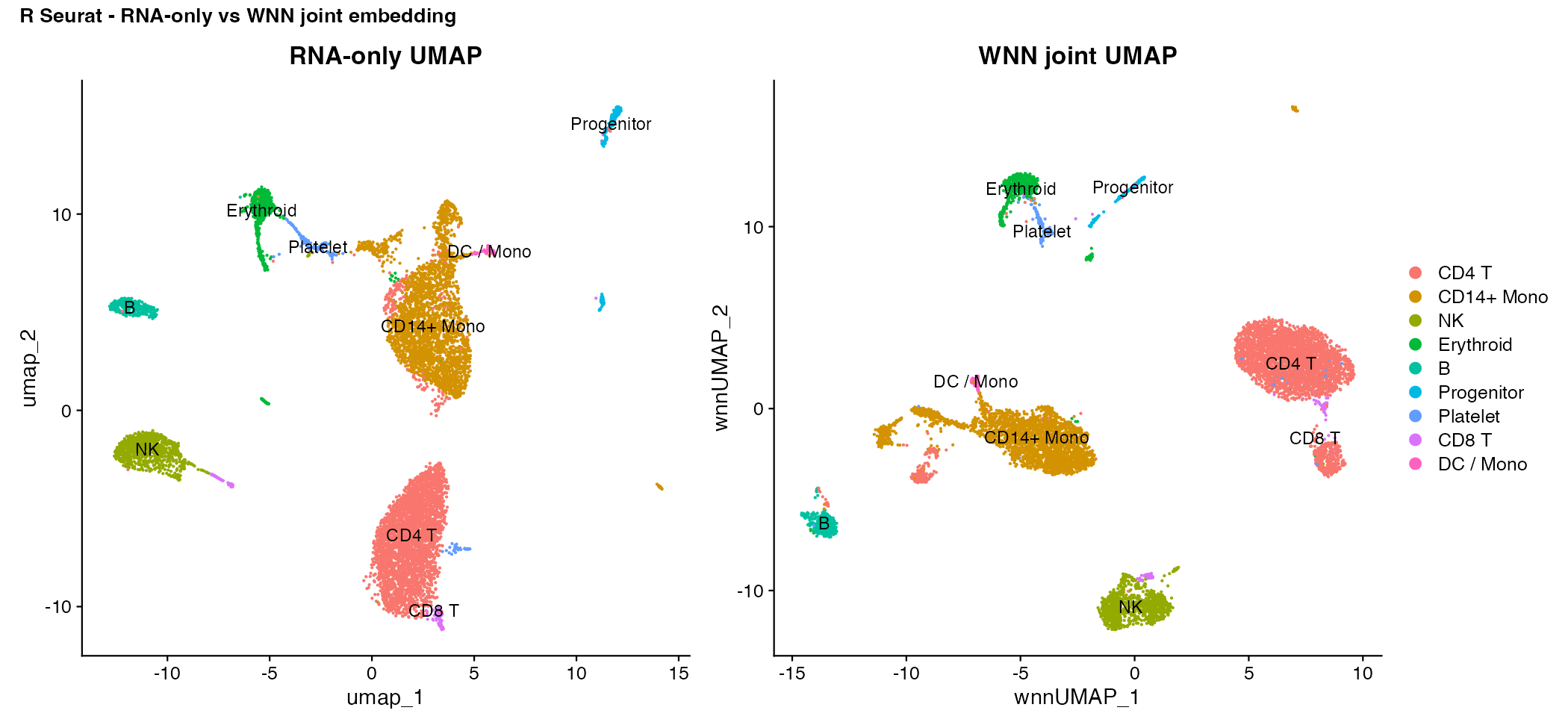
08_wnn_umap_clusters.png is the joint embedding. The comparison that matters is 09_wnn_vs_rna_umap.png — the same cells with the same labels, embedded on RNA alone (left) and on the joint graph (right):

R (Seurat)	Python (Truecell)

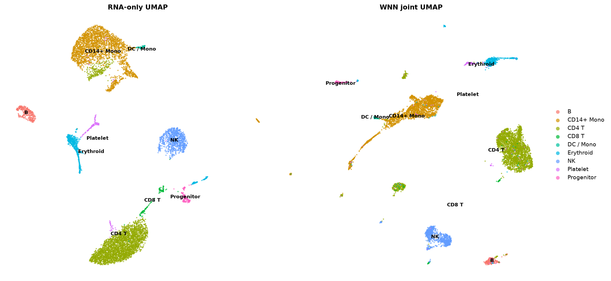UMAP has no canonical rotation, so don't read the orientation — read which populations form their own islands. Both sides resolve CD4 T, CD14+ Mono, NK and B as separate territories, with erythroid/platelet/progenitor grouped away from the immune lineages.

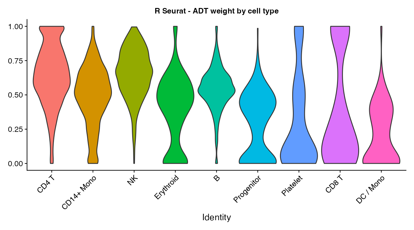
10_adt_weight_by_celltype.png plots the weights themselves. The violins are bimodal against the 0 and 1 rails rather than a bump at 0.5 — individual cells commit, and the per-type mean is a summary of that split, not a description of a typical cell:

R (Seurat)	Python (Truecell)

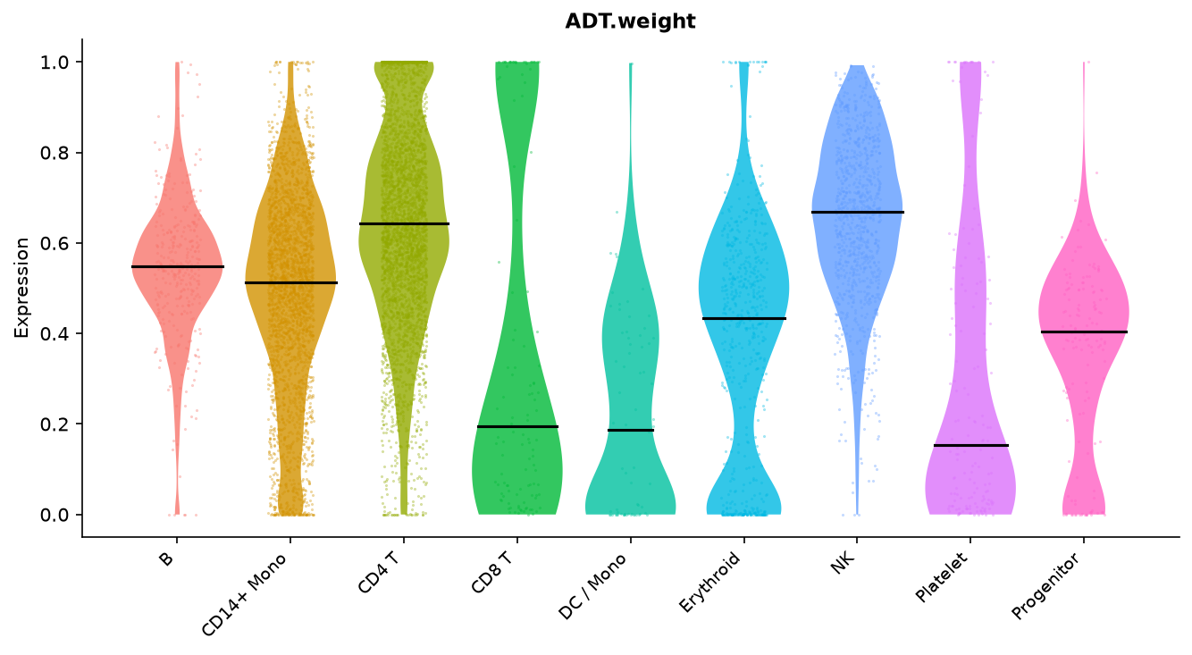The two panels are drawn to be read against each other. Both put the cell types in the same order and give each one the same colour, taken from Seurat's hue_pal over all twelve labels annotate_cells can return. Both mark the median, which vln_plot always draws and the R script adds, and neither draws points. R has one more violin: its clustering finds a 69-cell DC / Mono cluster, and Truecell's puts the same 69 cells in CD14+ Mono. The colours are spread over the whole list, so the type Truecell lacks moves no other colour.

ADT.weight is a metadata column, not a gene, but vln_plot resolves it the same way Seurat's VlnPlot does. Both panels label the axis ADT weight rather than the generic Expression.

The whole flow is wrapped as run_wnn(obj) in cbmc_citeseq_tutorial.py; run_full() prints the WNN cluster count and the mean modality weights per cell type.

How close is this to Seurat?¶

Close, and now measured rather than asserted. --report compares three things against a live Seurat 5.5.1 run:

Quantity	Agreement
ADT CLR — per-protein mean · sd · min · max	max abs diff 4.9e-15 (no RNG anywhere in it)
WNN modality weight, per cell on 8,617 shared barcodes	Pearson 0.9838 · Spearman 0.9812 · median abs diff 0.0161
Mean ADT weight, whole panel	0.5539 against 0.5556 — relative 3.1e-03
Cell-type label, per cell	98.72% concordant (8,507 / 8,617)
WNN clusters · cells · genes · proteins	21 · 8,617 · 20,379 · 13 — all identical
RNA clusters	15 against Seurat's 16: truecell's graph folds Seurat's 69-cell DC/Mono cluster into CD14+ Mono

The progenitor gap was never a WNN difference. This section used to record progenitor at 0.06 away from Seurat while every other type agreed to 0.02, and attributed it to cluster boundaries. The per-cell dump settled it: re-grouping truecell's own weights by R's labels read 0.283 against R's 0.285. The weights agreed; the two tools put different cells in the bucket.

cell type	truecell	R	truecell's weights, R's labels	n (py / R)
Progenitor	0.352	0.285	0.283	146 / 184
Erythroid	0.378	0.397	0.400	606 / 566
every other type	—	—	moved by ≤0.003	—

Those two rows were the same disagreement seen from both ends: 61 cells on the progenitor/erythroid boundary landed differently, which barely moved erythroid's 600-cell mean and visibly moved progenitor's 150-cell one. That is a small-population effect on an annotation threshold, not a modality-weighting difference — and it is the kind of thing a per-cell-type summary table can never distinguish, which is why the handoff is keyed by barcode. With Seurat's optimiser on both sides the progenitor side of that boundary lands alike, 184 cells each, and truecell's own progenitor label reads 0.283 against Seurat's 0.282. Erythroid is 568 cells against 593.

The residual cause is the graph each tool builds. Seurat's exact (rann) neighbours give the same 16 RNA clusters as its default annoy search, so the difference sits upstream of the neighbour search, in the embedding. Both sides run the same CLR and the same annotate_cells thresholds, shared verbatim between the two scripts.

This table used to look much worse, and the cause was not in the WNN code. Truecell's CLR had its margin flag inverted relative to Seurat: margin=2 computed what Seurat's margin=1 computes and vice versa, so the protein matrix feeding apca — and therefore every weight — was the wrong transform. The published numbers ran 0.10–0.74 against R's 0.21–0.65, and erythroid and platelet sat at 0.62/0.53 against R's 0.40/0.30, on the protein side despite having no antibody in the panel. That inversion is fixed; the annotation thresholds in cbmc_citeseq_tutorial.py and cbmc_citeseq_verify.R had been retuned around it and are now shared verbatim. The bug survived because its unit test verified the CLR kernel but derived the axis mapping in Python rather than checking it against R — right formula, assumed axis. The guard that replaces it (test_clr_margin_matches_r_ground_truth) pins both margins to fixed output from a real Seurat run.

API Translation (multimodal additions)¶

Task	R (Seurat)	Python (Truecell)
Load CITE-seq	`read.csv` + `CollapseSpeciesExpressionMatrix`	`cbmc_citeseq()`
Add a 2^nd assay	`cbmc[["ADT"]] <- CreateAssayObject(counts)`	`obj.assays["ADT"] = create_assay5_object(counts, key="adt_")`
CLR-normalise protein	`NormalizeData(..., method="CLR", margin=2)`	`normalize_data(..., normalization_method="CLR", margin=2)`
Switch modality	`DefaultAssay(cbmc) <- "ADT"` / `adt_`/`rna_` keys	`feature_plot(..., assay="ADT")`
WNN neighbours	`FindMultiModalNeighbors(reduction.list, dims.list)`	`find_multi_modal_neighbors(obj, reduction_list, dims_list)`
Cluster on joint graph	`FindClusters(graph.name = "wsnn")`	`find_clusters(obj, graph_name="wsnn")`
UMAP on joint graph	`RunUMAP(nn.name = "weighted.nn")`	`run_umap(obj, graph="wsnn")`

References¶

Stoeckius M, Hafemeister C, Stephenson W, Houck-Loomis B, Chattopadhyay PK, Swerdlow H, Satija R, Smibert P (2017). Simultaneous epitope and transcriptome measurement in single cells. Nature Methods 14, 865–868. https://doi.org/10.1038/nmeth.4380

Hao Y, Hao S, Andersen-Nissen E, et al. (2021). Integrated analysis of multimodal single-cell data. Cell 184, 3573–3587. https://doi.org/10.1016/j.cell.2021.04.048 (WNN)

Seurat multimodal vignette: https://satijalab.org/seurat/articles/multimodal_vignette Seurat WNN vignette: https://satijalab.org/seurat/articles/weighted_nearest_neighbor_analysis