The Object Model Itself — R Seurat vs Truecell (Python)

Every other tutorial in this series compares an algorithm: does run_pca land where RunPCA lands, does hto_demux call the same cells. This one compares the container — the accessors, the layer machinery and the bookkeeping that Seurat's own command cheat sheet is made of. Every R Seurat call is paired with the Truecell equivalent and both outputs are shown side by side.

Dataset: PBMC 3k — 2,700 cells × 13,714 genes (10x Genomics), the same object used in the guided tutorial and Tutorial T-dr. Auto-downloads (~24 MB). R reference: Seurat 5.5.1 / SeuratObject 5.4.0 · Python: Truecell

Seurat	Truecell
Cells(obj) / Features(obj)	cells(obj) / features(obj)
Layers(obj) / LayerData(obj, "data")	layers(obj) / layer_data(assay, "data")
obj[["RNA"]] <- split(obj[["RNA"]], f = batch)	assay.split_layers(batch)
JoinLayers(obj)	assay.join_layers()
DefaultAssay(obj) / Key(obj[["RNA"]])	default_assay(obj) / key(assay)
Embeddings / Loadings / Stdev	embeddings / loadings / stdev
FetchData(obj, c("CD3E", "PC_1"))	fetch_data(obj, ["CD3E", "PC_1"])
Idents / WhichCells / RenameIdents / subset	idents / which_cells / rename_idents / subset
Command(obj)	[c.key for c in obj.commands]

This tutorial found and fixed eleven defects. The layered assay's split / JoinLayers pair was not a round trip — it returned the right numbers in the wrong columns, silently. FetchData returned sparse-matrix objects instead of expression values. The command log had never been wired up at all. The findings are written up below with before-and-after behaviour, and all eleven are fixed in the same pull request as this tutorial.

---

Why this is the sharpest net in the series

Almost nothing here is stochastic. Cell orders, layer names, matrix dimensions, key strings, non-zero counts and command names either match R exactly or they are wrong — 89 of the 91 anchors are compared with no tolerance at all. The other tutorials have to argue about whether a 2 % gap is RNG or a bug; this one mostly does not have that conversation.

That matters because the object layer is where a defect is quietest. A broken run_pca shows up in a plot. A broken JoinLayers returns a matrix of exactly the right shape, full of exactly the right numbers, in the wrong order.

---

Headline

Anchor	Result
Anchors matching Seurat exactly	91 / 91
Cells — count and order (md5 of the barcode vector)	identical (e9278a0983c2)
Features — count and order	identical, 13,714
Variable features — the shared 2,000-gene basis	identical (fbd5a143114e)
Layers and their dimensions	counts 13714×2700 · data 13714×2700 · scale.data 2000×2700 — all match
Assay key / PCA key	rna_ / PC_ — match
Metadata columns	orig.ident, nCount_RNA, nFeature_RNA — match
nCount_RNA total	6,386,518 on both
Identities (marker-gated)	T 1300 · Mono 788 · B 322 · Other 290 — match
WhichCells(idents = "T") — count and order	1,300, identical vector
subset(idents = "Mono")	788 cells × 13,714 features — match
FetchData — CD3E column total	2,831.901591 on both
split → JoinLayers round trip	identity — name, cell order and matrix all restored
Command log	5 entries, NormalizeData.RNA … FindNeighbors.RNA.pca — match
PCA standard deviations	agree to ~4e-4 relative (randomized SVD vs irlba)
kNN / SNN graph edges	RNA_nn 54,000 = 2,700 × 20 and RNA_snn 199,616 on both

---

Setup

Both tools read the same 10x directory, and the Python run writes the cell barcodes and variable features it used so the R script rests on an identical basis. If the two disagree about which cells or genes are in play, nothing below is interpretable.

R (Seurat)

Python (Truecell)

library(Seurat) counts <- Read10X(data.dir = DATA) obj <- CreateSeuratObject( counts = counts, project = "pbmc3k_objects", min.cells = 3, min.features = 200) hvg <- gsub("_", "-", readLines("figures_objects/hvg_features.txt")) obj <- NormalizeData(obj, verbose = FALSE) obj <- FindVariableFeatures(obj, nfeatures = 2000, verbose = FALSE) VariableFeatures(obj) <- hvg obj <- ScaleData(obj, features = hvg, verbose = FALSE) obj <- RunPCA(obj, features = hvg, npcs = 20, verbose = FALSE) obj <- FindNeighbors(obj, dims = 1:10, verbose = FALSE)

from truecell.truecell import create_truecell_object from truecell.datasets import pbmc3k counts, genes, cells = pbmc3k() obj = create_truecell_object( counts=counts, assay="RNA", project="pbmc3k_objects", min_cells=3, min_features=200, feature_names=list(genes), cell_names=list(cells)) normalize_data(obj) find_variable_features(obj, nfeatures=2000) hvg = list(obj.assays["RNA"].variable_features) scale_data(obj, features=hvg) run_pca(obj, n_pcs=20, features=hvg) find_neighbors(obj, dims=list(range(10)))

Gotcha, and it is not truecell's. Read10X rewrites _ to - in gene symbols — pbmc3k carries Y_RNA and a long tail of RP11-*_* — while truecell's loader leaves them alone. That belongs to the two file readers, not to the object model, so feature names are compared in R's spelling on both sides rather than failing every field that mentions a gene.

---

Who is in the object

R (Seurat)	Python (Truecell)
dim(obj) # 13714 2700 head(Cells(obj), 3) # AAACATACAACCAC-1 ... Assays(obj) # "RNA" DefaultAssay(obj) # "RNA" Key(obj[["RNA"]]) # "rna_" colnames(obj[[]]) # orig.ident nCount_RNA nFeature_RNA	len(obj.cell_names()), len(obj.feature_names()) # 2700, 13714 G.cells(obj)[:3] # ['AAACATACAACCAC-1', ...] obj.assay_names() # ['RNA'] obj.default_assay # 'RNA' G.key(obj.get_assay()) # 'rna_' obj.meta_data.columns # orig.ident, nCount_RNA, nFeature_RNA

Order is compared, not just membership: the tutorial fingerprints the barcode vector with an order-sensitive md5, and both sides return e9278a0983c2.

---

Layers — the v5 architecture

The single biggest change from Seurat v4, and the part that had never been run.

R (Seurat)

Python (Truecell)

Layers(obj) # "counts" "data" "scale.data" dim(LayerData(obj[["RNA"]], "scale.data")) # 2000 2700 # Split the assay by a grouping factor batch <- ifelse(seq_len(ncol(obj)) %% 2 == 1, "batch1", "batch2") split_assay <- split(obj[["RNA"]], f = batch) Layers(split_assay) # "counts.batch1" "counts.batch2" # ...and put it back joined <- JoinLayers(split_assay) Layers(joined) # "counts" identical(colnames(LayerData(joined, "counts")), colnames(obj)) # TRUE

assay = obj.get_assay("RNA") assay.layers_list() # ['counts', 'data', 'scale.data'] assay.layer_data("scale.data").shape # (2000, 2700) # Split the assay by a grouping factor batch = batch_labels(len(obj.cell_names())) split_assay = assay.split_layers(batch, layer="counts") split_assay.layers_list() # ['counts.batch1', 'counts.batch2'] # ...and put it back joined = split_assay.join_layers() joined.layers_list() # ['counts'] joined.cells("counts") == assay.cells() # True

The batch column is assigned deterministically (alternating cells), not with sample() as Seurat's vignette does, so both tools split on identical membership and any difference downstream belongs to the layer code rather than to two different random draws.

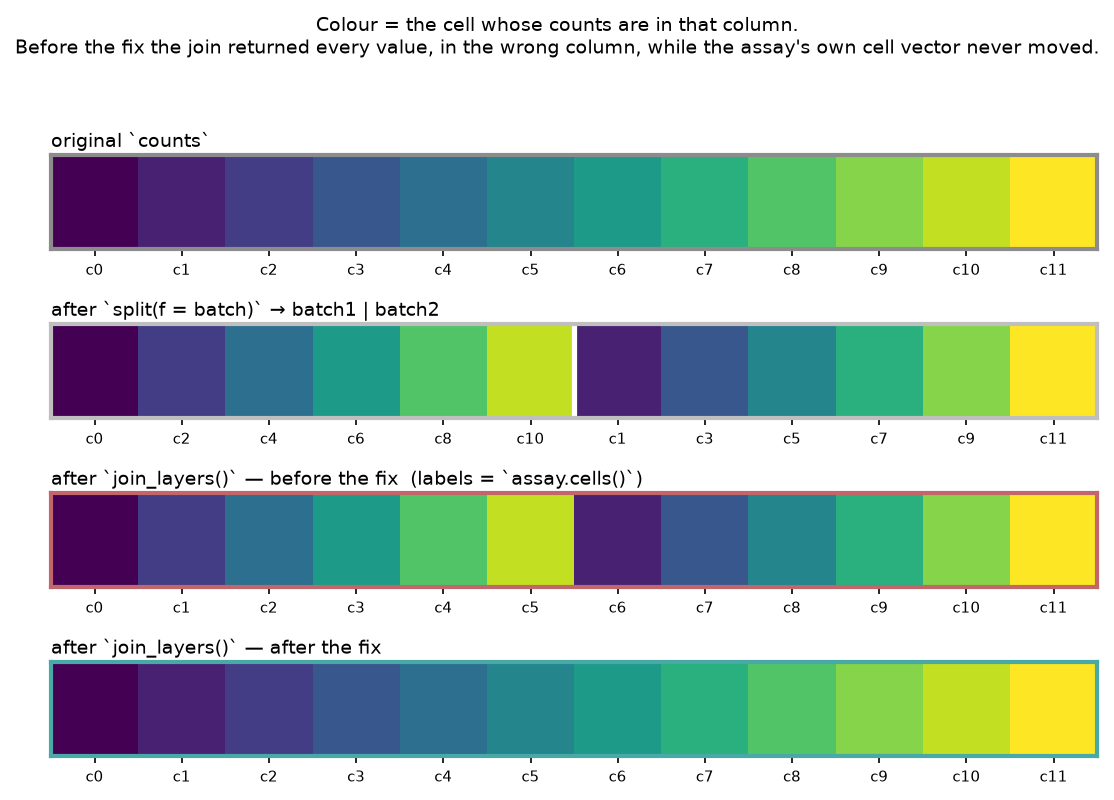
This is where the tutorial earned its keep. Before the fix, that last comparison was False, and nothing said so:

---

Reductions, graphs and FetchData

R (Seurat)

Python (Truecell)

Reductions(obj) # "pca" Key(obj[["pca"]]) # "PC_" dim(Embeddings(obj[["pca"]])) # 2700 20 dim(Loadings(obj[["pca"]])) # 2000 20 round(Stdev(obj[["pca"]])[1:3], 4) # 6.9345 4.4608 3.8388 Graphs(obj) # "RNA_nn" "RNA_snn" round(FetchData(obj, c("nCount_RNA", "CD3E", "PC_1"))[1:2, ], 6) # nCount_RNA CD3E PC_1 # AAACATACAACCAC-1 2419 2.226555 4.563726 # AAACATTGAGCTAC-1 4903 0.000000 0.247260

sorted(obj.reductions) # ['pca'] G.key(obj.reductions["pca"]) # 'PC_' G.embeddings(obj.reductions["pca"]).shape # (2700, 20) G.loadings(obj.reductions["pca"]).shape # (2000, 20) np.round(G.stdev(obj.reductions["pca"])[:3], 4) # [6.9344 4.4608 3.8386] list(obj.graphs) # ['RNA_nn', 'RNA_snn'] G.fetch_data(obj, ["nCount_RNA", "CD3E", "PC_1"]).head(2) # nCount_RNA CD3E PC_1 # AAACATACAACCAC-1 2419.0 2.226555 -4.549421 # AAACATTGAGCTAC-1 4903.0 0.000000 -0.233127

PC_1 is addressed by the reduction's Key, which is what Key() is for. CD3E agrees to the last digit shown — and to 2,831.901591 summed over all 2,700 cells.

PC_1 does not agree, and should not: a principal component's sign is arbitrary, so R's +4.563726 and truecell's −4.549421 are the same axis pointed opposite ways. That is why the tutorial compares the absolute column sum across tools, and pins the exact value only within one tool — a fetched embedding column must be the object's own embedding column, whatever the two PCAs did. The residual magnitude difference (~0.1 %) is the randomized SVD against irlba, which is T-dr's subject, not this one's.

---

Identities and the command log

R (Seurat)

Python (Truecell)

table(Idents(obj)) # B Mono Other T # 322 788 290 1300 length(WhichCells(obj, idents = "T")) # 1300 levels(Idents(RenameIdents(obj, "T" = "T_cell"))) # "B" "Mono" "Other" "T_cell" dim(subset(obj, idents = "Mono")) # 13714 788 names(obj@commands) # NormalizeData.RNA FindVariableFeatures.RNA # ScaleData.RNA RunPCA.RNA FindNeighbors.RNA.pca

ident_anchor(obj.idents)["counts"] # {'B': 322, 'Mono': 788, 'Other': 290, 'T': 1300} len(G.which_cells(obj, ident="T")) # 1300 sorted(set(obj.rename_idents({"T": "T_cell"}).idents)) # ['B', 'Mono', 'Other', 'T_cell'] len(obj.subset(idents="Mono").cell_names()) # 788 [c.key for c in obj.commands] # ['NormalizeData.RNA', 'FindVariableFeatures.RNA', # 'ScaleData.RNA', 'RunPCA.RNA', 'FindNeighbors.RNA.pca']

Identities come from marker-gene thresholds (CD3E → T, MS4A1 → B, LYZ → Mono, first gate wins) rather than from clustering, and for the same reason the batch split is deterministic: Louvain drifts by a cluster between the two tools, which would put noise into comparisons that are otherwise exact.

---

What this tutorial found

Eleven fidelity defects: five in the layered assay, three in FetchData, three in the object's bookkeeping. All are fixed in the same pull request.

1–5. split / JoinLayers was not a round trip

	before	after (and R)
layer name after join	joined	counts
cell order after join	c0 c2 c4 … c1 c3 c5	c0 c1 c2 …
matrix restored	✗	✓
join_layers() on a prepared assay	ValueError	works
split layer names	counts_batch1	counts.batch1
generics.split_layers	NotImplementedError	dispatches

The cell-order one is the serious one. The assay's own cell vector never moves during a split, so a join that returns the columns in split order leaves the matrix silently transposed against the metadata that indexes it — ask for cell c1's column and get c2's. Nothing raised, the shape was right, and every checksum was right, because every value was still present.

join_layers() with no arguments — R's idiom, and the only call a real script makes — additionally raised ValueError on any prepared assay, because it hstacked counts, data and a variable-features-only scale.data together regardless of their differing feature counts. The fix groups layers by the stem they were split from, and records that provenance at split time rather than parsing it back out of the name: Seurat's own scale.data contains the separator, so splitting on the last . would read it as layer scale of group data and rejoin it into something that never existed.

6–8. FetchData returned objects instead of numbers

np.asarray on a sparse matrix yields a 0-d object array wrapping it, not its contents, so .flatten() broadcast one csc_matrix down all 2,700 rows. Every cell's "expression" was a copy of the whole matrix. This is the most-called accessor in Seurat, on the default assay class.

It had a test. test_fetch_data asserted the column name and the row count — both of which a column of identical sparse matrices satisfies perfectly.

Two smaller gaps came with it: embedding columns could not be addressed by their Key (PC_1 raised KeyError), and an unqualified fetch read counts where R reads data, returning raw integers where every vignette shows normalized values. When there is no data layer, truecell now falls back to counts and warns, exactly as Seurat does.

9–11. The bookkeeping

log_truecell_command was a public export with zero call sites, so obj.commands was always empty. Seurat logs five entries for this pipeline. The log now records R's names (RunPCA.RNA, not run_pca.RNA) on the same reasoning that keeps layer names scale.data and reduction keys PC_: it is a lookup table users query, so it is data rather than decoration.

orig.ident — the first column of every Seurat object's metadata, and the default identity class — was never created. And add_meta_data rejected the plain vector that R's AddMetaData documents and every vignette passes it.

The two graph differences, since closed

This tutorial originally reported two neighbour-graph differences it declined to fix, on the grounds that they belonged to find_neighbors rather than the object model. Both were investigated and fixed in PR #55, and both are now exact:

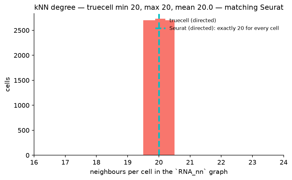
• find_neighbors stored a symmetrized kNN graph where Seurat's is directed, so its degree ran from 20 to 83 (mean 28.1, nnz 75,740) against Seurat's flat k.param. It now stores the directed graph — degree is exactly 20 for every cell and nnz is exactly 2,700 × 20 = 54,000, matching Seurat.
• The SNN dropped the self-edge Seurat keeps. It is now present on all 2,700 cells, and RNA_snn nnz is 199,616 on both sides.

One wrinkle is worth keeping, because it made the comparison lie for a while after the fix had landed. FindNeighbors defaults to nn.method = "annoy", which is approximate, while truecell's neighbour search is exact — so the two sides were building their graphs from different neighbour tables. That cost 182 SNN edges (199,434 against 199,616) and read as a truecell defect. This tutorial's R script now pins nn.method = "rann" so both sides use exact neighbours, and the graphs agree. If you change the neighbour method on one side only, expect this anchor to move.

---

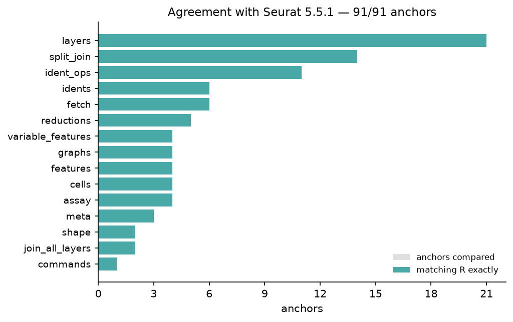
Parity — verified against R Seurat

Section	Anchors	Matching
layers (names, dims, nnz, sums, per-layer cells)	21	21
split_join (the round trip)	14	14
ident_ops (WhichCells, RenameIdents, subset)	11	11
idents	6	6
fetch (FetchData)	6	6
reductions	5	5
variable_features	4	4
features · cells · assay	4 each	4 each
graphs	4	4
meta	3	3
shape · join_all_layers	2 each	2 each
commands	1	1
Total	91	91

Every anchor is an exact match; the only tolerances applied anywhere are on the two fields that read a PCA, and they are named explicitly in FLOAT_TOLERANCES rather than applied across the board. The graphs row was 2 of 4 when this tutorial was written — see the two graph differences.

---

Running it

python tutorials/pbmc3k_objects_tutorial.py     # downloads ~24 MB on first run
Rscript tutorials/pbmc3k_objects_verify.R       # writes r_anchors.json
python tutorials/pbmc3k_objects_tutorial.py     # now prints the side-by-side table
python tutorials/generate_objects_plots.py      # figures

The R script needs Seurat, SeuratObject, Matrix, jsonlite and digest. Run the Python side first: it publishes the shared variable-feature and cell lists the R script reads back.