Cell Hashing — Demultiplexing pooled samples (R Seurat vs Truecell)¶

A side-by-side port of Seurat's hashing vignette. Cell Hashing (Stoeckius et al. 2018) tags each sample with a distinct antibody-conjugated oligo — a hashtag (HTO) — before pooling many samples on one droplet lane. Every droplet then carries, on top of its mRNA, a barcode of hashtag counts saying which sample it came from. Demultiplexing turns that back into a per-cell call: a singlet from sample 3, a doublet of samples 1 and 2, or a negative empty-ish droplet.

Truecell ships both of Seurat's demultiplexers, and this walkthrough runs them against their R references on byte-identical input:

hto_demux ↔ HTODemux — a negative-binomial cutoff per hashtag, learned from the tag's background cluster.
multiseq_demux ↔ MULTIseqDemux — a kernel-density cutoff per barcode instead (McGinnis et al.).

Why this tutorial exists. Every hashing feature landed after PR #10 and had only ever been checked against synthetic fixtures. This is the first time hto_demux / multiseq_demux meet real data with a Seurat reference — a direct test of the CLR-margin fix (#32) and the clara k-medoids default (#34). The target is R-vs-Python call concordance, not a headline cell count.

The data — a raw barnyard, not the vignette's filtered PBMC¶

The vignette downloads a pre-filtered pbmc_umi_mtx.rds from Dropbox — an R binary with no clean cross-language form. So truecell.datasets.pbmc_hashing uses the original GEO matrices (GSE108313) instead, which both languages read identically. Two consequences worth stating up front:

These are raw, unfiltered barcodes. The list is dominated by empty-ish droplets, so the Negative rate is high (~42 %). That is expected and does not affect the R-vs-Python comparison — both tools see the same droplets.
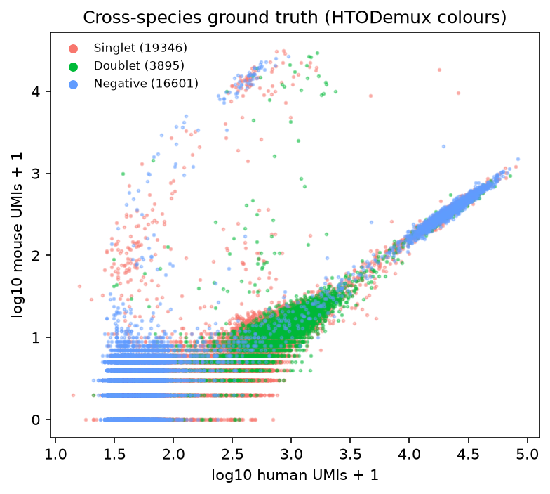
The RNA is aligned to a combined human + mouse genome. That is deliberate: a droplet with both human and mouse transcripts is a species-mixed multiplet no hashtag was consulted for — an independent doublet signal (used in Step 5).

40,899 genes × 39,842 cells   ·   8 hashtags: BatchA … BatchH

Step 1 · Load, build the object, attach & CLR-normalise the HTO assay¶

Hashtag counts are compositional, so they are centered-log-ratio (CLR) normalised — margin 1 (per hashtag across cells), which is Seurat's default and what the hashing vignette uses. Both demultiplexers read that normalised layer.

R (Seurat) Python (Truecell)

# HTODemux needs only the HTO assay; the RNA text is
# ~41k x 50k dense (~13 GB), so read just its header
# for the barcode set the Python loader intersects to.
hdr <- readLines(gzfile(RNA_TSV), n = 1)
rna_cells <- strsplit(hdr, "\t")[[1]][-1]

hto <- read.csv(gzfile(HTO_CSV), row.names = 1,
                check.names = FALSE)
hto <- hto[!rownames(hto) %in%
           c("bad_struct","no_match","total_reads"), ]
common <- intersect(rna_cells, colnames(hto))
hto <- as.matrix(hto[, common])
rownames(hto) <- sub("-.*$", "", rownames(hto))

obj <- CreateSeuratObject(counts = as.sparse(hto),
                          assay = "HTO")
obj <- NormalizeData(obj, assay = "HTO",
        normalization.method = "CLR", margin = 1)

from truecell.datasets import pbmc_hashing
from truecell.truecell import create_truecell_object
from truecell.assay5 import create_assay5_object
from truecell.preprocessing import normalize_data

# downloads ~34 MB, drops the 3 QC rows, aligns
# the RNA and HTO matrices on shared barcodes
rna, genes, hto, hto_names, cells = pbmc_hashing()

obj = create_truecell_object(counts=rna, assay="RNA",
        min_cells=3, feature_names=genes, cell_names=cells)
obj.assays["HTO"] = create_assay5_object(
        counts=hto, feature_names=hto_names,
        cell_names=cells, key="hto_")
normalize_data(obj, assay="HTO",
        normalization_method="CLR", margin=1)

The tutorial shortens each hashtag name (BatchA-AGGACCATCCAA → BatchA) on both sides so names, hash.ID values and plot labels line up. The R reference reads only the RNA header because the dense RNA text would need ~13 GB in memory — and the RNA has no bearing on the hashtag calls anyway.

Step 2 · HTODemux — negative-binomial threshold per hashtag¶

R (Seurat) Python (Truecell)

obj <- HTODemux(obj, assay = "HTO",
                positive.quantile = 0.99)
table(obj$HTO_classification.global)
#  Doublet Negative  Singlet
#     3916    16575    19351

from truecell.hto import hto_demux

hto_demux(obj, assay="HTO",
          positive_quantile=0.99, normalize=False)
obj.meta_data["HTO_classification.global"].value_counts()
#  Singlet     19346
#  Negative    16601
#  Doublet      3895

Global class	Truecell	R Seurat
Singlet	19,346	19,351
Doublet	3,895	3,916
Negative	16,601	16,575

The eight samples come out balanced (Truecell hash.ID): BatchA 2,470 · BatchB 2,807 · BatchC 2,529 · BatchD 2,305 · BatchE 2,080 · BatchF 2,089 · BatchG 2,465 · BatchH 2,601.

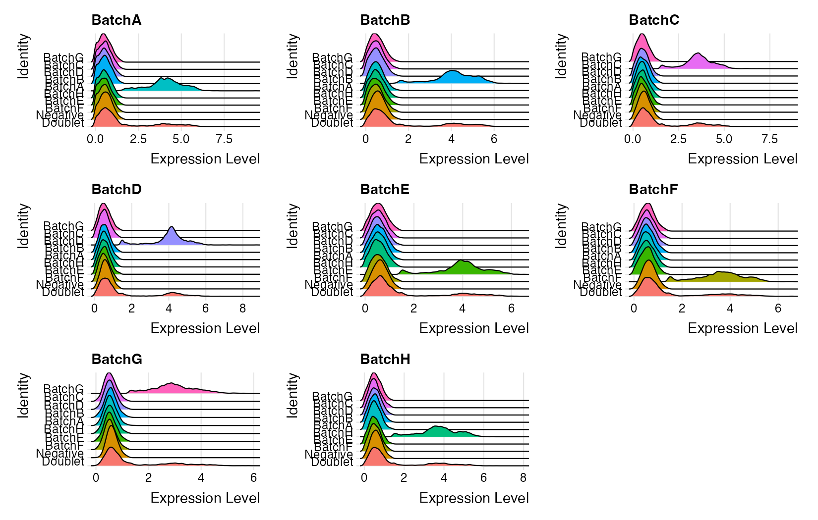
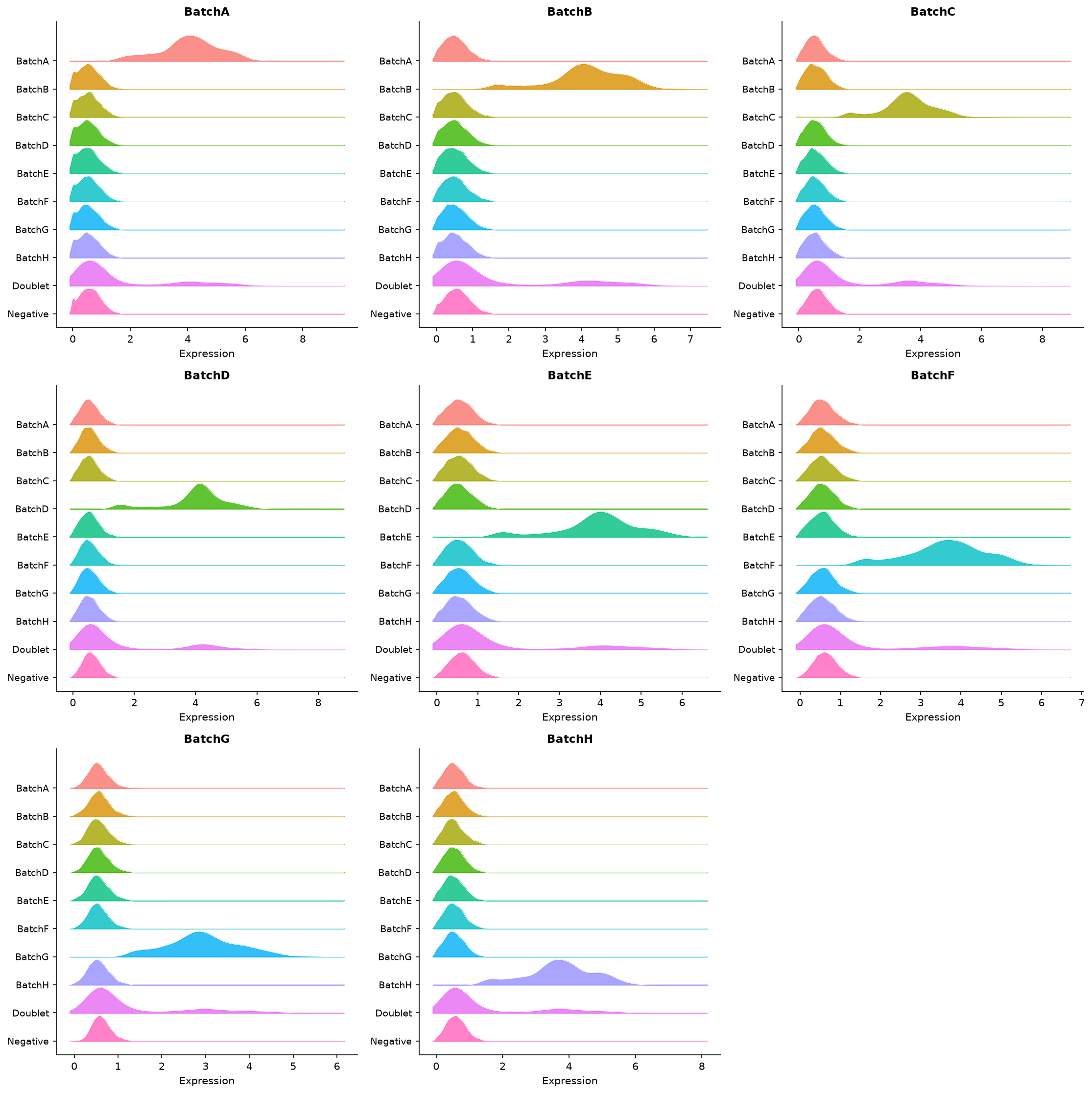
The ridge plot is the canonical QC read: each hashtag lights up only in the sample it was assigned to; the Doublet row shows elevated background, the Negative row sits at zero.

R — `RidgePlot`	Truecell — `ridge_plot`

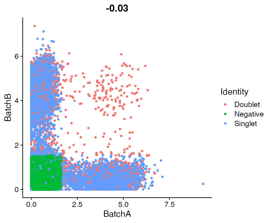
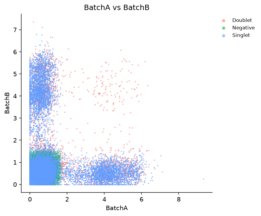
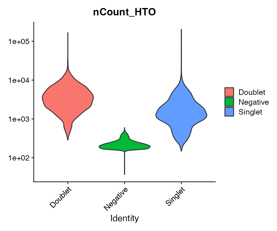
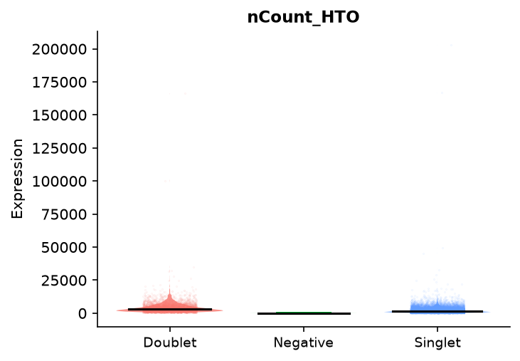
Two hashtags against each other separate the singlet arms (on the axes) from the doublet cloud (interior); total hashtag counts run higher for doublets.

R — `FeatureScatter`	Truecell — `feature_scatter`

R — `VlnPlot(nCount_HTO)`	Truecell — `vln_plot("nCount_HTO")`

Step 3 · MULTIseqDemux — kernel-density threshold per barcode¶

Same normalised input, a different rule for the cutoff: a Gaussian KDE over each barcode's values, thresholded between its background and positive modes.

R (Seurat) Python (Truecell)

obj <- MULTIseqDemux(obj, assay = "HTO",
                     quantile = 0.7)
#  Singlet 16388 · Negative 21231 · Doublet 2223

from truecell.multiseq import multiseq_demux

multiseq_demux(obj, assay="HTO",
               quantile=0.7, normalize=False)
#  Singlet 17644 · Negative 19560 · Doublet 2638

The two methods agree strongly on the confident calls — every HTODemux Negative is a MULTIseq Negative, and the singlet blocks overlap almost entirely — but MULTIseq is the more conservative of the two here (more Negatives, fewer Doublets).

Step 4 · Cross-species ground truth¶

Because the RNA is a combined human+mouse alignment, a droplet's species mix is a doublet signal the hashtags never saw. pbmc_hashing splits the genes by symbol case (all-upper = human, title-case / …Rik / mt- = mouse) and labels each cell human / mouse / mixed.

HTODemux species	human	mixed	mouse
Singlet	19,055	218	73
Doublet	3,832	45	18
Negative	15,799	734	68

Read this honestly: of 997 species-mixed droplets, HTODemux calls only 45 Doublet — most (734) are Negative. At raw-barcode depth the mixed pool is dominated by low-count ambient droplets, not genuine two-cell doublets, so this is a weak sanity check, not a clean doublet benchmark. It confirms the pipeline runs on real barnyard data; it does not adjudicate the demux calls.

The headline · R-vs-Python call concordance¶

Every cell, compared call-for-call against the Seurat reference on identical input (report_concordance() reads the r_calls.csv the verify script writes):

Comparison	Agreement
HTODemux global class (Singlet/Doublet/Negative)	99.81 %
HTODemux sample assignment (`hash.ID`)	99.81 %
MULTIseqDemux call (`MULTI_ID`)	94.67 %

HTODemux global — Truecell (rows) × R (cols):

	R Doublet	R Negative	R Singlet
Doublet	3,889	0	6
Negative	0	16,566	35
Singlet	27	9	19,310

HTODemux reproduces Seurat to 99.81 % — just 77 of 39,842 cells differ, for both the global class and the per-sample assignment. That residual is clara's sampling nondeterminism (R and Python draw different sub-samples and neither can seed the other — see truecell._clara), comfortably inside the ~1 % the docstring promises. This is the confirmation the initiative was built to get: the CLR fix (#32) and the clara default (#34) hold up against real Seurat.

MULTIseqDemux agrees on 94.67 % — materially lower, and legitimately so. Both tools threshold the same CLR values (HTODemux at 99.81 % proves the input and alignment are identical), so the gap is entirely in the KDE step: scipy's gaussian_kde and R's density() differ in bandwidth selection and grid construction. It does not reduce to a single knob — swapping scipy's default bandwidth for R's nrd0 (with R's 512-point grid) moves concordance the wrong way, so faithfully matching R would mean reproducing R's whole density estimator, not tuning one parameter. The practical takeaway: HTODemux is the more cross-tool-reproducible of the two demultiplexers, and a ~5 % MULTIseq disagreement at the margins is a genuine method-implementation difference, logged here rather than papered over.

Running it yourself¶

python tutorials/pbmc_hashing_tutorial.py     # downloads ~34 MB, prints the report
Rscript tutorials/pbmc_hashing_verify.R       # Seurat reference → r_calls.csv + r_*.png
python tutorials/pbmc_hashing_tutorial.py     # re-run: now prints the R-vs-Python concordance
python tutorials/generate_hashing_plots.py    # Truecell figures → figures_hashing/py_*.png

Figures (tutorials/figures_hashing/, r_* = R Seurat, py_* = Truecell):

Figure	Description
`py_01_ridge.png`	Hashtag CLR enrichment per assigned sample
`py_02_scatter.png`	Two hashtags, coloured by HTODemux global class
`py_03_ncount_violin.png`	Total hashtag counts per global class
`py_04_species_scatter.png`	Human vs mouse UMIs — the barnyard ground truth

R Seurat → Truecell API¶

Task	R (Seurat)	Python (Truecell)
CLR-normalise hashtags	`NormalizeData(obj, assay="HTO", method="CLR", margin=1)`	`normalize_data(obj, assay="HTO", normalization_method="CLR", margin=1)`
Demultiplex (HTODemux)	`HTODemux(obj, assay="HTO", positive.quantile=0.99)`	`hto_demux(obj, assay="HTO", positive_quantile=0.99)` — both default `kfunc="clara"`
Demultiplex (MULTI-seq)	`MULTIseqDemux(obj, assay="HTO", quantile=0.7)`	`multiseq_demux(obj, assay="HTO", quantile=0.7)`
Global class	`obj$HTO_classification.global`	`obj.meta_data["HTO_classification.global"]`
Sample assignment	`obj$hash.ID`	`obj.meta_data["hash.ID"]`

Reference¶

Stoeckius M, Zheng S, Houck-Loomis B, et al. (2018) Cell Hashing with barcoded antibodies enables multiplexing and doublet detection for single cell genomics. Genome Biology 19, 224. https://doi.org/10.1186/s13059-018-1603-1