SCTransform Tutorial — R Seurat vs Truecell (Python)¶

A Python port of Seurat's sctransform vignette on the PBMC 3k dataset. SCTransform replaces the NormalizeData → FindVariableFeatures → ScaleData trio with a single regularized negative-binomial model: counts are modelled per gene as a function of cell sequencing depth, the per-gene parameters are smoothed across genes, and the model's Pearson residuals become the normalized values. The vignette's point is that this removes technical effects more effectively, so — run over more PCs (dims 1:30) — it resolves finer immune subsets.

Dataset: 3k PBMCs — 10x Genomics (2016) Python: Truecell v0.9.0

python tutorials/pbmc3k_sctransform_tutorial.py   # printed validation + the model handoff
python tutorials/generate_sctransform_plots.py    # writes figures_sctransform/  (Truecell)
Rscript tutorials/pbmc3k_sctransform_verify.R     # R figures + r_sct_model.csv / r_anchors.json
python tutorials/pbmc3k_sctransform_tutorial.py --report   # the side-by-side, gene by gene

Most R figures below link the canonical Seurat vignette images; the two the vignette omits (cell-type UMAP, SCT-vs-standard) are generated locally by pbmc3k_sctransform_verify.R.

Step 1 · Load data & QC metric¶

R (Seurat) Python (Truecell)

library(Seurat)
pbmc_data <- Read10X("pbmc3k/filtered_gene_bc_matrices/hg19/")
pbmc <- CreateSeuratObject(counts = pbmc_data)
pbmc <- PercentageFeatureSet(pbmc, pattern = "^MT-",
                             col.name = "percent.mt")

from truecell.datasets import pbmc3k
from truecell.truecell import create_truecell_object
from truecell.preprocessing import percentage_feature_set

counts, genes, cells = pbmc3k()
pbmc = create_truecell_object(counts=counts, assay="RNA", min_cells=3,
                            min_features=200, feature_names=genes,
                            cell_names=cells, project="pbmc3k")
percentage_feature_set(pbmc, pattern=r"^MT-", col_name="percent.mt")

Step 2 · SCTransform (one call replaces three)¶

SCTransform regresses percent.mt out of the residuals and returns 3,000 variable features in a new SCT assay.

R (Seurat) Python (Truecell)

pbmc <- SCTransform(pbmc, vars.to.regress = "percent.mt",
                    verbose = FALSE)
# -> 3000 variable features, assay "SCT"

from truecell.sctransform import sctransform

sctransform(pbmc, vars_to_regress=["percent.mt"], n_features=3000)
# -> obj.assays["SCT"] with counts / data / scale.data layers
#    3000 variable features; SCT is now the active assay

Truecell's sctransform follows R's algorithm step for step, in pure NumPy: a vectorised per-gene GLM, theta.ml for the NB dispersion, and regularization of the parameters across genes by Nadaraya–Watson smoothing against the log10 geometric mean, with a Sheather–Jones bandwidth. Like Seurat 5 it defaults to vst.flavor="v2" (vst_flavor="v2") — depth slope fixed at log(10), non-overdispersed genes modelled as pure Poisson, and a variance floor — with vst_flavor="v1" available for the original 2019 model. scale.data holds the clipped Pearson residuals for the 3,000 variable features (a genuine feature-subset layer).

Step 3 · PCA → UMAP → clustering over 30 PCs¶

R (Seurat) Python (Truecell)

pbmc <- RunPCA(pbmc, verbose = FALSE)
pbmc <- RunUMAP(pbmc, dims = 1:30)
pbmc <- FindNeighbors(pbmc, dims = 1:30)
pbmc <- FindClusters(pbmc)            # resolution 0.8
DimPlot(pbmc, label = TRUE)

from truecell.reduction import run_pca
from truecell.neighbors import find_neighbors
from truecell.clustering import find_clusters
from truecell.umap import run_umap

run_pca(pbmc, n_pcs=50, features=pbmc.assays["SCT"].variable_features)
find_neighbors(pbmc, dims=range(30), k_param=20)
find_clusters(pbmc, resolution=0.8, random_seed=0)
run_umap(pbmc, dims=range(30), seed=42)

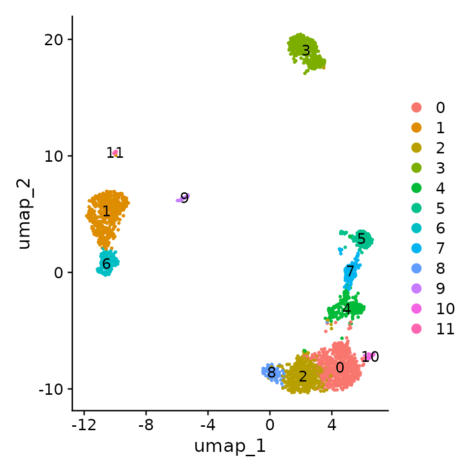
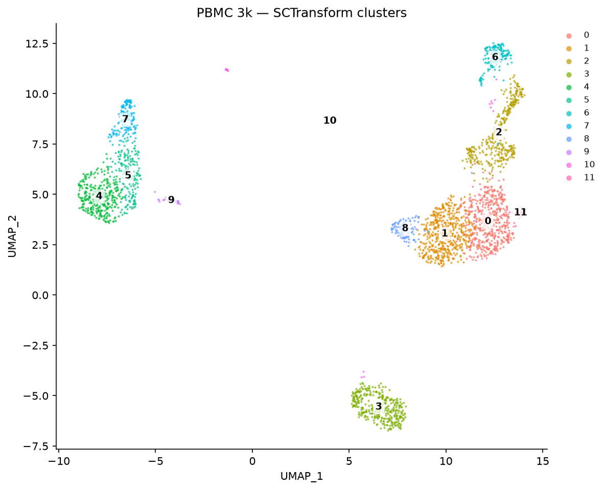
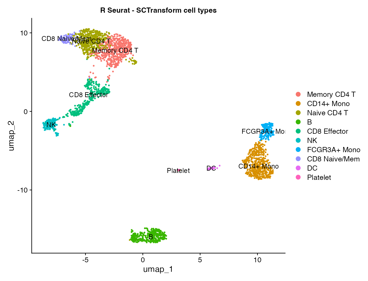
The T-cell mass resolves as a cytotoxicity gradient — Naive CD4 → Memory CD4 → CD8 Effector → NK — alongside two monocyte types, B cells, DC/pDC, and platelets. Annotating by relative marker enrichment gives:

R (Seurat)	Python (Truecell)

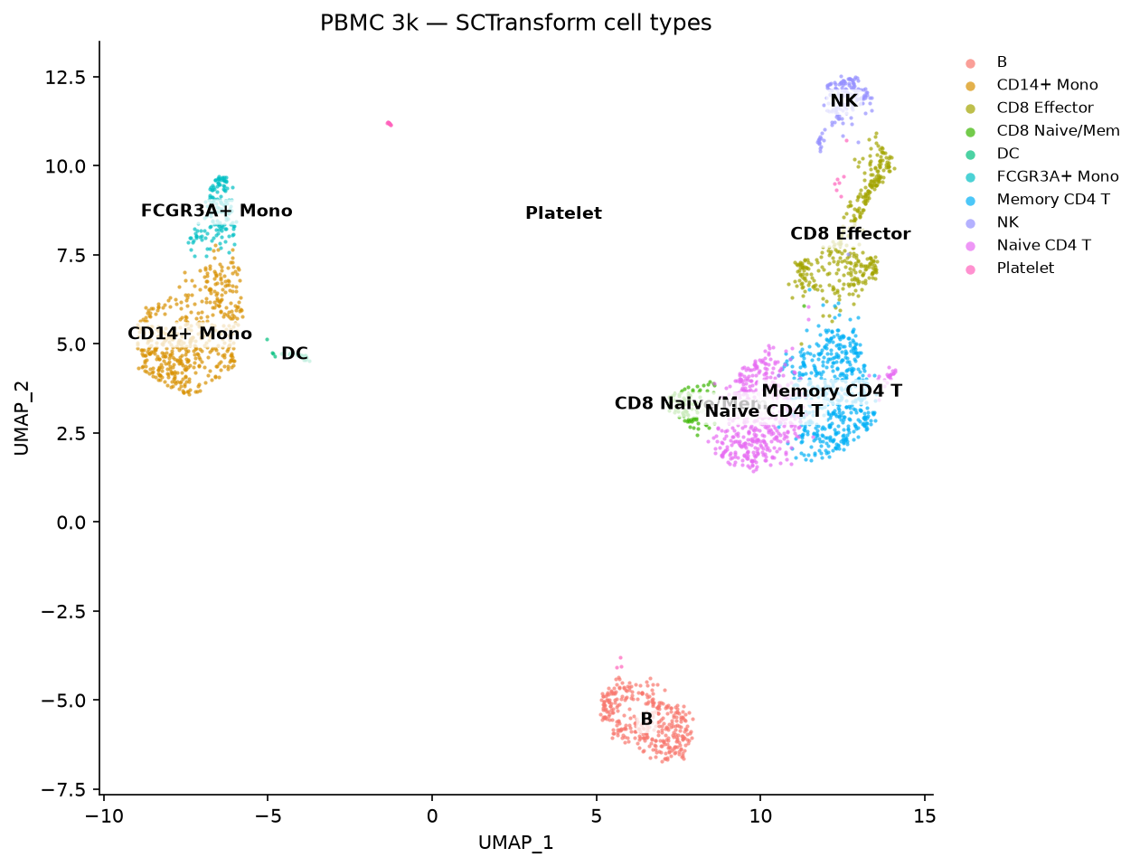The published Seurat vignette stops at clusters and prints no cell-type-annotated plot, so the R panel is generated by pbmc3k_sctransform_verify.R: the same SCT workflow, annotated by the same relative marker-enrichment rule Truecell uses. Both resolve the fine T subsets SCTransform is meant to sharpen.

Step 4 · Marker feature plots (the vignette panels)¶

R (Seurat) Python (Truecell)

FeaturePlot(pbmc, features = c("CD8A","GZMK","CCL5",
                               "S100A4","ANXA1","CCR7"), ncol = 3)
FeaturePlot(pbmc, features = c("CD3D","ISG15","TCL1A",
                               "FCER2","XCL1","FCGR3A"), ncol = 3)

from truecell.plotting import feature_plot

feature_plot(pbmc, ["CD8A","GZMK","CCL5","S100A4","ANXA1","CCR7"],
             reduction="umap", assay="SCT", ncol=3,
             min_cutoff="q05", max_cutoff="q95")
feature_plot(pbmc, ["CD3D","ISG15","TCL1A","FCER2","XCL1","FCGR3A"],
             reduction="umap", assay="SCT", ncol=3,
             min_cutoff="q05", max_cutoff="q95")

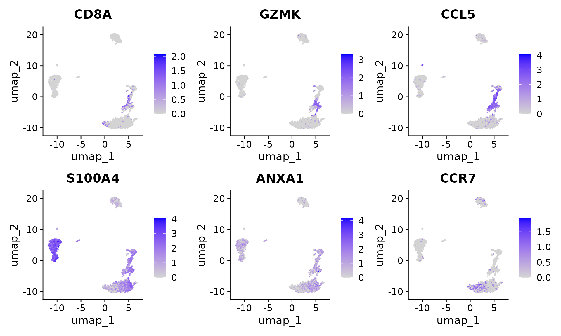
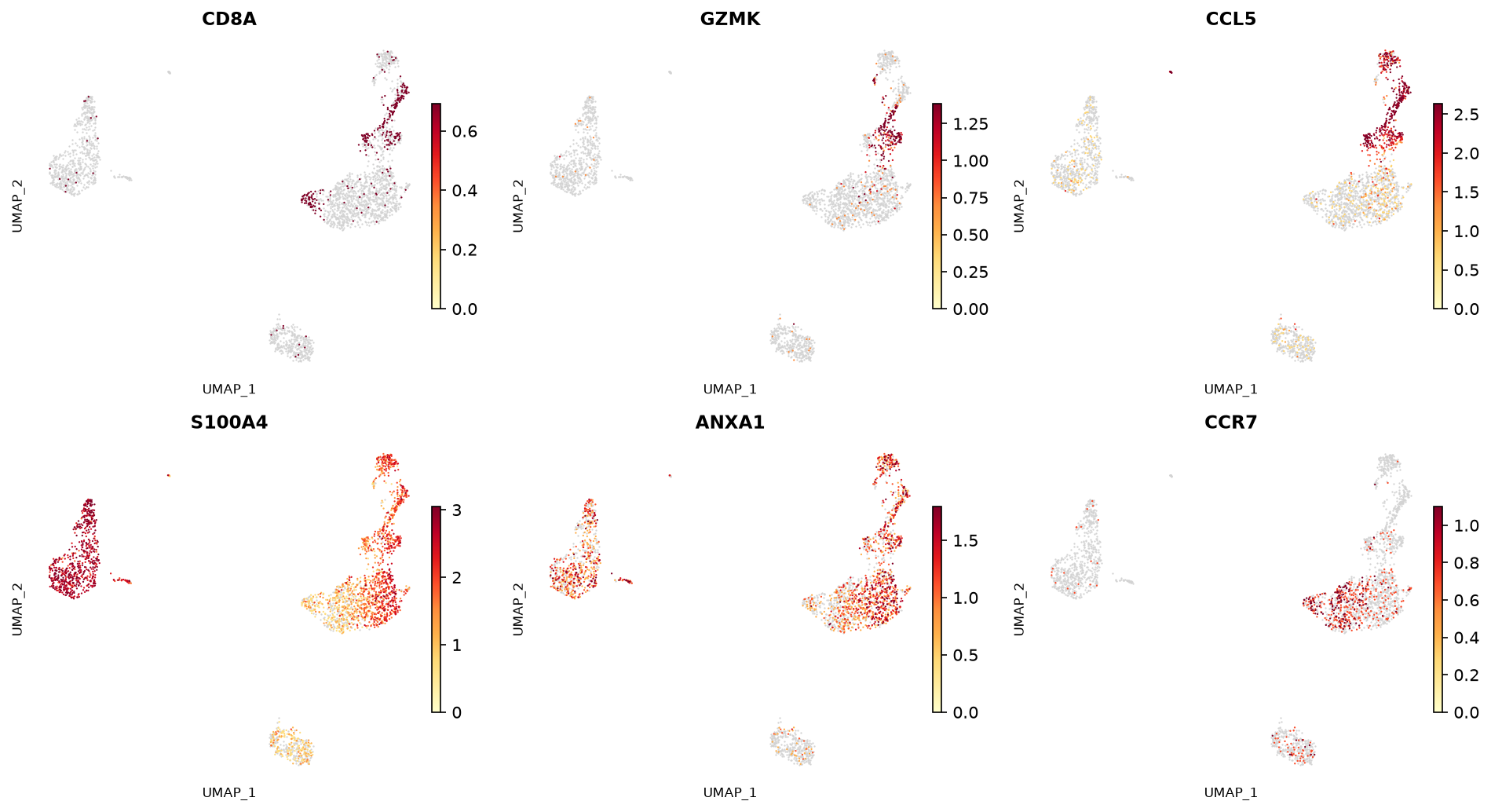
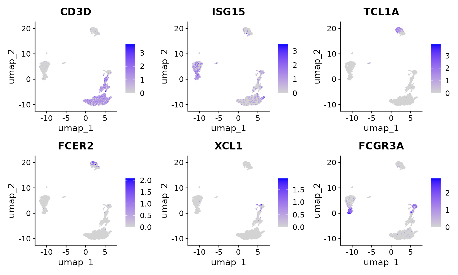
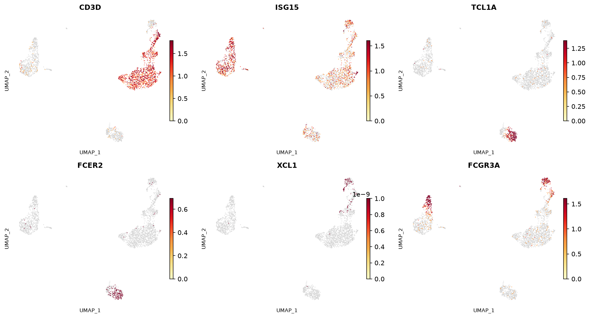
CD8A/GZMK/CCL5 mark the CD8 effector tip; CCR7 marks the naive end; S100A4/ANXA1 mark memory T cells; FCGR3A marks the CD16⁺ monocytes and NK; TCL1A/FCER2 pick out B-cell sub-structure — matching the vignette.

Step 5 · Violin plots¶

R (Seurat) Python (Truecell)

VlnPlot(pbmc, features = c("CD8A","GZMK","CCL5","S100A4",
        "ANXA1","CCR7","ISG15","CD3D"), pt.size = 0.2, ncol = 4)

from truecell.plotting import vln_plot
vln_plot(pbmc, ["CD8A","GZMK","CCL5","S100A4","ANXA1","CCR7","ISG15","CD3D"],
         group_by="sct_clusters", assay="SCT", ncol=4, pt_size=2.0)
# pt_size overlays jittered cells, matching R's VlnPlot(pt.size = 0.2);
# matplotlib sizes points by area, so the numeric value differs.

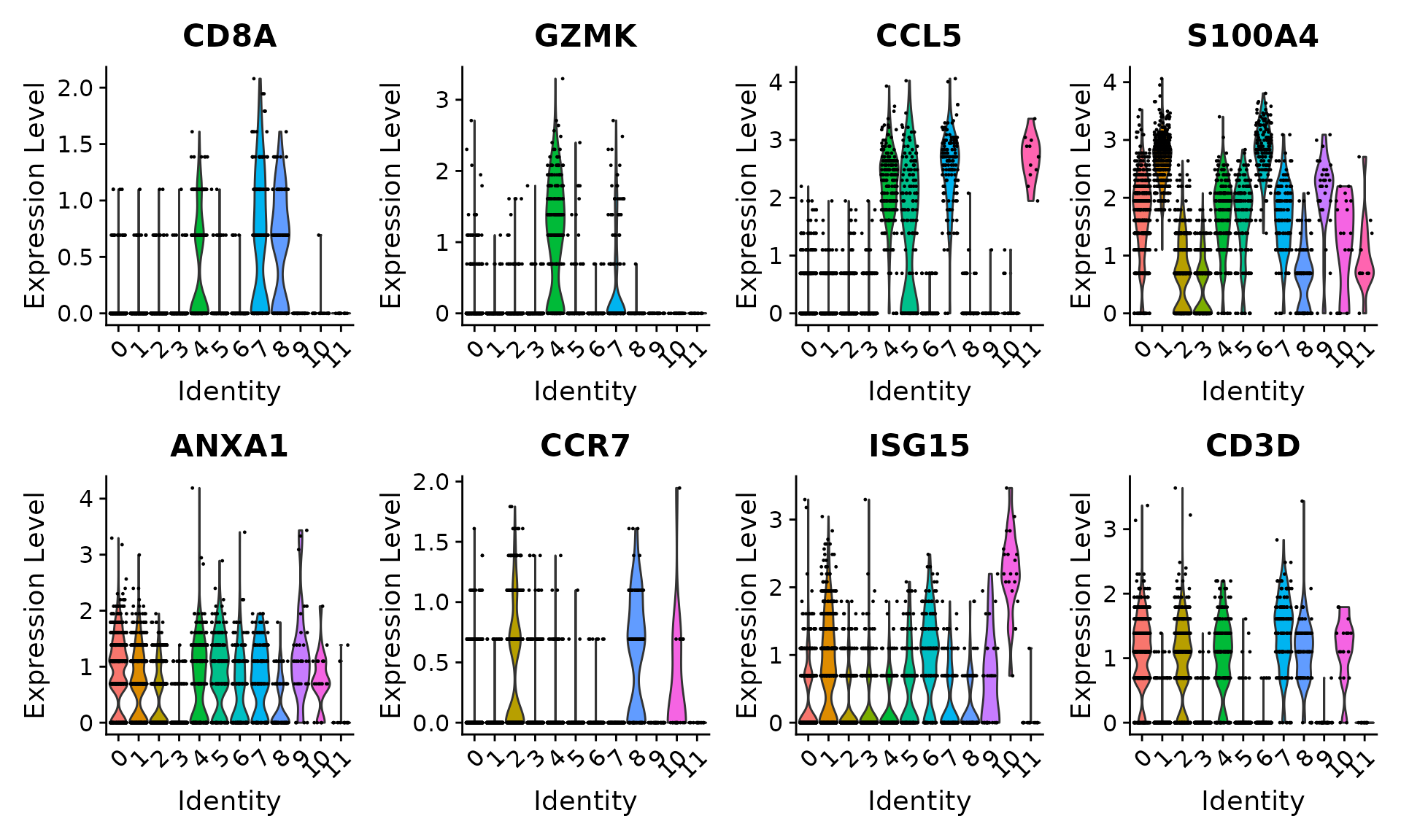
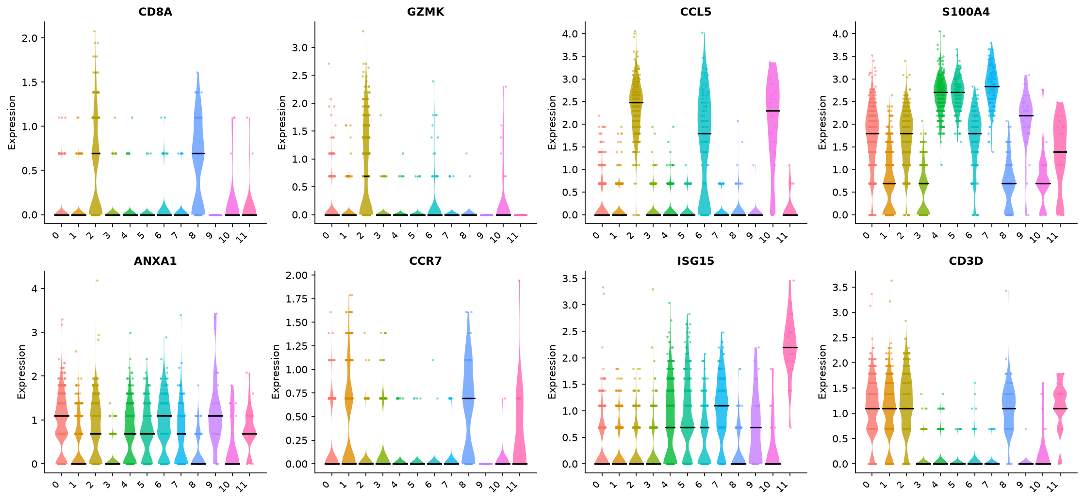
Both panels plot the SCT data layer (log1p of corrected counts) — R's VlnPlot default for an SCT assay — with cells jittered over each violin. The distributions track gene-for-gene: CD8A/GZMK spike on the cytotoxic CD8 cluster, CCL5 across the CD8/NK end, CD3D over all T clusters, CCR7 low and naive-restricted. The x-axes differ by one column — Truecell resolves 13 clusters (0–12) here versus the vignette's 12 (0–11) — and cluster numbering is not shared across the two plots anyway, so compare the per-gene shapes, not column positions. (See the accuracy note below.)

Step 6 · SCTransform vs standard log-normalization¶

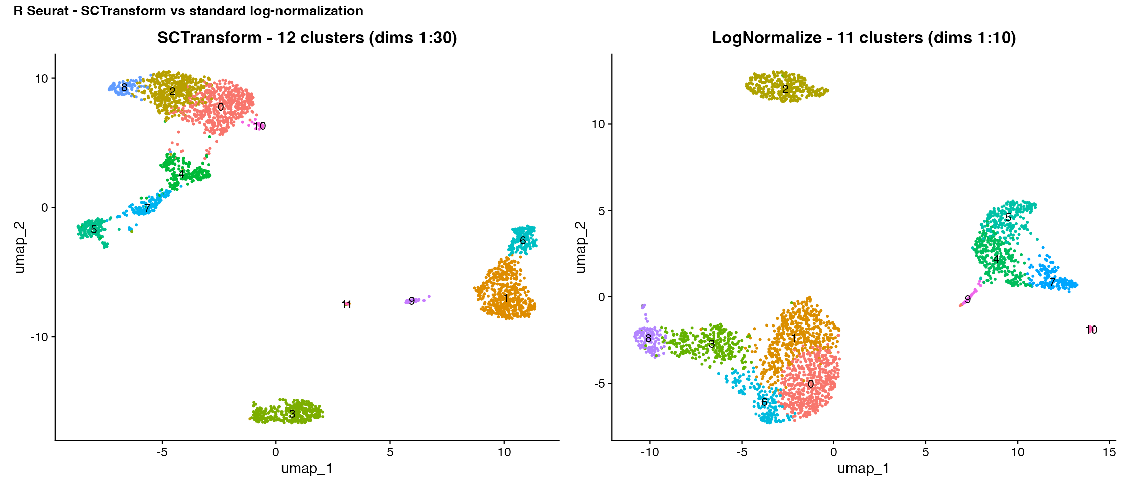
The published Seurat vignette does not include this comparison figure, but both toolkits can produce it — running SCTransform (dims 1:30) and LogNormalize (dims 1:10) on the same cells and rendering them side by side for a direct view of the resolution difference:

R (Seurat)	Python (Truecell)

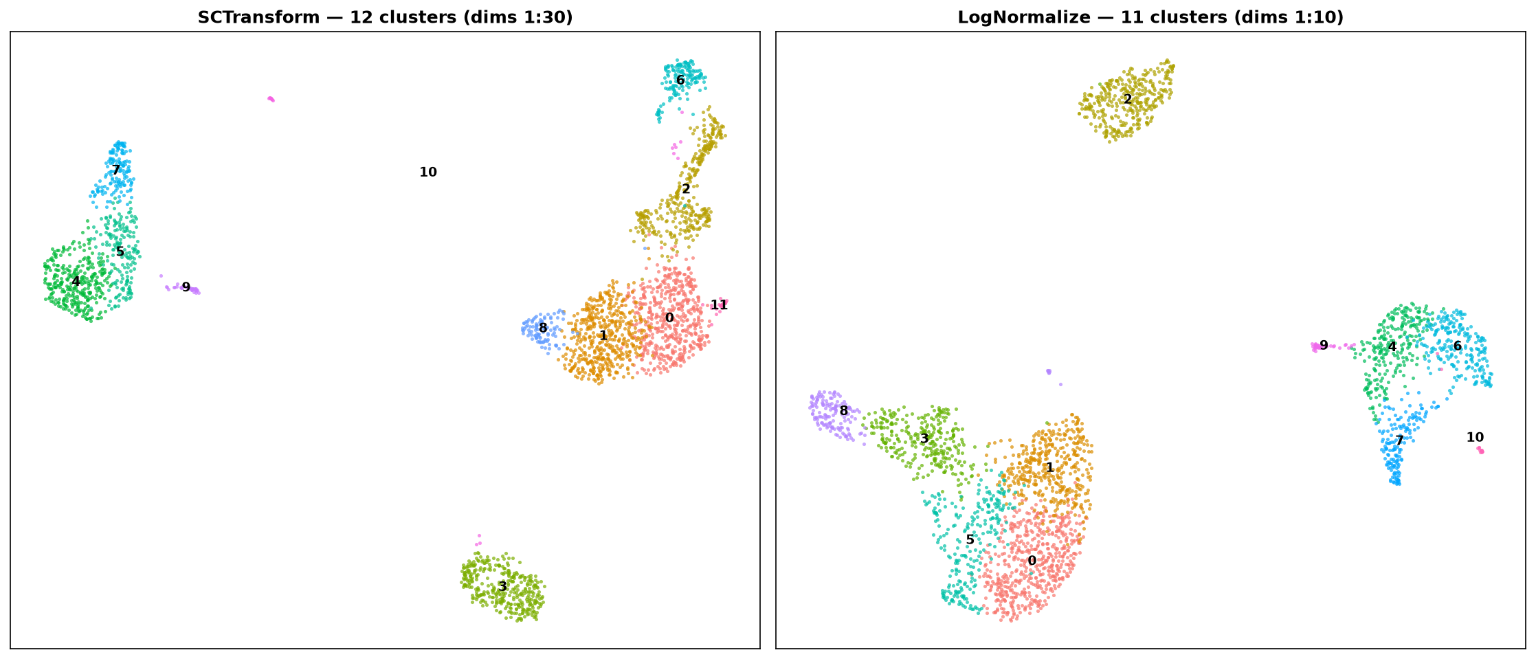Each panel: left = SCTransform (dims 1:30), right = LogNormalize (dims 1:10). The R panels come from pbmc3k_sctransform_verify.R.

Accuracy vs the R vignette¶

Aspect	R Seurat (vignette)	Truecell	Match
Normalization model	NB Pearson residuals	NB Pearson residuals	✅
Variable features	3,000	3,000	✅
PCs used	30 (dims 1:30)	30 (dims 1:30)	✅
`vars.to.regress`	`percent.mt`	`percent.mt`	✅
Major populations	T, NK, B, 2× Mono, DC, platelet	all recovered	✅
CD8 effector split (CCL5/GZMK) from CD4	yes	yes	✅
Naive vs memory CD4 (CCR7 vs S100A4)	yes	yes	✅
`vst.flavor` default	v2	v2	✅
Resolves more than log-norm	yes (the vignette's claim)	yes — 12 vs 11	✅
Clusters at resolution 0.8	12 (live run; vignette prints none)	12	✅
Clusters, LogNormalize arm	11	11	✅
Variable features shared with R	3,000	2,913 (97.1%)	✅
Regularized theta vs R (Spearman)	—	1.0000 over the 8,724 finite thetas	✅
Genes v2 calls non-overdispersed	3,848	3,848 — the same genes (Jaccard 1.0000)	✅
Regularized intercept vs R (Spearman)	—	1.0000	✅
Residual variance vs R (Spearman)	—	0.9986 (Pearson 0.9996)	✅
`detection_rate` · `gmean` vs R	—	max abs diff 5.0e-16 · 1.2e-12	✅
Residual clips (`sqrt(N)` · `sqrt(N/30)`)	±51.9615 · ±9.4868	identical	✅

These numbers are reproduced, not recorded. Everything in the table above comes out of a comparison you can re-run:

python tutorials/pbmc3k_sctransform_tutorial.py      # writes py_sct_model.csv + py_anchors.json
Rscript tutorials/pbmc3k_sctransform_verify.R        # writes r_sct_model.csv  + r_anchors.json
python tutorials/pbmc3k_sctransform_tutorial.py --report

The R script dumps Seurat's own SCTModel.list[[1]]@feature.attributes — the fitted model, per gene — and truecell stores the same eight columns under the same names on the SCT assay's meta_data, so the two tables line up directly. That matters more here than anywhere else in the series: this model was once wrong in four separate ways at once and the tutorial still drew a perfectly plausible UMAP. A picture cannot fail; a Spearman of −0.89 can.

Where it matches. The model, the 3,000 variable features, the 30-PC embedding, and the biology all reproduce: the CD8-effector / CD4 / NK split and the marker patterns the vignette highlights are all recovered. Against a live Seurat 5.5.1 / sctransform 0.4.3 run on the same cells, detection_rate and gmean agree to machine precision, the regularized intercept and theta both rank identically (Spearman 1.0000), the 3,848 genes v2 declares non-overdispersed are exactly the same genes on both sides, and both arms of the workflow now land on the same cluster counts — 12 under SCTransform, 11 under LogNormalize.

Where it differs. Two places, both small and both expected. Residual variance ranks at Spearman 0.9986 rather than 1, which moves 87 of the 3,000 variable features (98 of the top 100 still agree); vst samples its 2,000 step-1 genes at random, so R does not reproduce itself across seeds here either. And residual_mean is the one column that does not track by rank — Spearman 0.71 against Pearson 0.99. It is also the one column nothing downstream reads: Seurat records it but selects features on residual_variance. The rank disagreement sits entirely in genes whose residual mean is ~1e-3 or smaller, which is numerical dust on residuals that range to ±52.

The ±1 cluster gap this section used to describe is closed. It read "13 against R's 12" for a long time, attributed to the RNG and to the different clustering libraries. Both arms now agree exactly. What changed was not SCTransform but the graph underneath it — PR #55 stored Seurat's directed kNN graph, restored the SNN self-edge and added GroupSingletons.

This was wrong until recently. Truecell used to resolve 9 clusters here — fewer than log-normalization's 11, which inverts the vignette's entire point. A moment estimator stood in for theta.ml, the regularization smoothed against the arithmetic rather than geometric gene mean and targeted log(theta) rather than the overdispersion factor, and residual variance was computed from residuals clipped at sqrt(N/30) instead of sqrt(N). The result flattened every residual: the regularized theta came out anti-correlated with R's (Spearman −0.89) and only 414 of 3,000 variable features agreed. See the CHANGELOG and tests/test_sctransform_r_fidelity.py.

API Translation (SCTransform additions)¶

Task	R (Seurat)	Python (Truecell)
SCTransform	`SCTransform(obj, vars.to.regress="percent.mt")`	`sctransform(obj, vars_to_regress=["percent.mt"])`
Model flavor	`SCTransform(obj, vst.flavor="v2")` (default)	`sctransform(obj, vst_flavor="v2")` (default)
Use SCT assay	`DefaultAssay(obj) <- "SCT"` (automatic)	active assay set to `"SCT"` automatically
Variable features	`VariableFeatures(obj)`	`obj.assays["SCT"].variable_features`
Residuals	`GetAssayData(obj, "scale.data")`	`obj.assays["SCT"].layers["scale.data"]`
Per-gene model fit	`SCTResults(obj, slot="feature.attributes")`	`obj.assays["SCT"].meta_data` (`theta`, `residual_variance`, `gmean`)

References¶

Hafemeister C, Satija R (2019). Normalization and variance stabilization of single-cell RNA-seq data using regularized negative binomial regression. Genome Biology 20, 296. https://doi.org/10.1186/s13059-019-1874-1

Choudhary S, Satija R (2022). Comparison and evaluation of statistical error models for scRNA-seq. Genome Biology 23, 27. (sctransform v2)

Seurat sctransform vignette: https://satijalab.org/seurat/articles/sctransform_vignette